Further Properties of Space-filling Curves

This is the final part of a three-part post. For the first, see here.

In the previous post, we examined an iterative sequence of curves, the limit of which after an infinite number of iterations is called the Hilbert curve. We now prove that the Hilbert curve indeed has the property it was constructed to have: it fills the unit square. Consider the first iteration again.



The first iteration includes all four points of the form (m/2,n/2) when m and n are each either one or three. In binary decimal notation, 1/4 = 0.01 and 3/4 = 0.11. To see the relevance of this fact, now consider the second iteration.



The points along the curve marked by black dots are of the form (m/8,n/8) with m and n both odd (and between 0 and 8), and two of these points are explicitly marked with their coordinates for clarity. It is obvious that the second iteration contains all points of this form. In binary notation, the points are of the form (0.ab1,0.cd1), where a, b, c, and d can stand for either 0 or 1. For example, (7/8,5/8) = (0.111,0.101). Since each iteration contains smaller copies of the previous one, it is clear that this pattern continues, and the third iteration will include all points of the form (m/16,n/16), with 0 < m, n < 16 and both m and n odd. In decimal notation, the curve includes all points each of whose coordinates has a 4-digit terminating binary expansion that ends in 1 (just as the second iteration had 3-digit terminating binary expansions ending in 1).

Next, we must note that any binary expansion can be approximated to arbitrary accuracy by others ending in the digit "1". For example, let P be the point in the unit square (0.101010101...,0.10100000...), where the repetition in the first expansion continues infinitely. Now consider the sequence {(0.11,0.11), (0.101,0.101),(0.1011, 0.1011),(0.10101,0.10001),...}. The nth point in this sequence lies on the curve of the nth iteration, and the sequence converges to the point P defined above. Thus the point P lies on the limit of the iterations, i.e., the Hilbert Curve itself. Note that the second coordinate of point P is exactly matched by the point on the 2nd iteration, and the sequence goes on to actually veer away (temporarily) from its final value. However, it still approaches the same limit as the sequence continues.

Since binary is simply another way of writing the real numbers, it is easy to show that there is a binary expansion for every real number from 0 to 1. For more discussion on this topic, see The Infinity Series, specifically here. Therefore, the Hilbert Curve visits every point in (and on) the unit square, and is indeed a space-filling curve. We note next that the Hilbert curve actually "overachieves" its goal; it actually visits several points of the unit square multiple times. For example, the point (1/2,1/2) is the limit of the sequence {(0.11,0.11), (0.101,0.101),(0.1001, 0.1001),(0.10001,0.10001),...} as well as of another sequence {(0.01,0.01), (0.011,0.011),(0.0111, 0.0111),(0.01111,0.01111),...}. Thus the function mapping the unit interval onto the Hilbert Curve is not one-to-one though it is continuous. Contrast this with the first function we constructed from the unit interval onto the unit square, which was one-to-one (after resolving the issue of multiple decimal representations) but not continuous.

It is impossible for a function from the unit interval to the unit square to be one-to-one and continuous. Such functions are called homeomorphisms, and two spaces for which is it possible to construct a homeomorphism mapping one onto the other are topologically equivalent in a certain sense. This means that they share certain intrinsic toplogical properties. For example, if a homeomorphism from a space that is connected (see image below) to another space exists, the latter space must also be connected.

Examples of connected and disconnected spaces.    Connected spaces can only have one component (A),  while  disconnected ones have multiple disjoint components (B).

Also, two homeomorphic spaces (this means that there is a homeomorphism from one onto the other) share other connectedness properties. For example, the unit interval has the property that, when any point of it (except an endpoint) is removed, it becomes disconnected. However, the unit square cannot be disconnected by the removal of any single point. Hence the two spaces differ in a topological property that is conserved by homeomorphisms and are not homeomorphic. Therefore, a continuous space-filling curve that is also one-to-one is impossible.

It is also worth noting that the concept of a Hilbert curve can be extended to any finite dimension; in three dimensions, instead of filling the unit square, the curve fills the unit cube. This would be done by dividing the cube into 2³ = 8 cubes of side length 1/2 and divding the unit interval into 8 corresponding subintervals for the first iteration, and so on. Generally, the Hilbert curve, like many other mathematical oddities, shatters our intuition when it comes to what properties mathematical objects can possess, and reminds us of the differences between the physical and mathematical worlds.

Sources: Counterexamples in Analysis by Bernard R. Gelbaum and John M. H. Olmsted, Space-filling Curve on Wikipedia, http://upload.wikimedia.org/wikipedia/commons/9/95/Connected_and_disconnected_spaces.svg

Constructing a Space-filling Curve

This is the second part of a three-part post. For the first, see here.

The previous post introduced the concept of a curve in the plane, presenting it as a type of mapping from one-dimensional to two-dimensional space, with the added condition that it be continuous. Finally, an interesting mapping that fills the unit square was presented. However, this example is not continuous. To show this, we shall demonstrate that a particular sequence {x_n} = {x₁,x₂,x₃,...} of points in t-space (the one-dimensional domain of the mapping) converges to a point x, also in the domain of f. Then, we shall show that the corresponding sequence of points {f(x₁),f(x₂),f(x₃),...} does not converge to the image f(x) of the limit of the sequence. This will prove that the mapping is discontinuous.

Let {x_n} be the sequence {0.490000...,0.499000...,0.499900...,...}. Clearly this sequence converges to x = 0.500. The sequence in the unit square {(0.400...,0.900...),(0.490...,0.900...),(0.490...,0.990...)}, whose members correspond to the value of f at each member of {x_n} converges to (0.500...,0.999...), but the value of f at x is not this value. Rather it is f(0.500...) = (0.500...,0.000...). Thus f is not a continuous mapping. Note that even if the non-terminating decimal expansions were selected for those members of the unit interval where there are two possibilities, the function would still be discontinuous, and one would this time use a sequence of points approaching t = 1/2 from above rather than below.

Though, as mentioned previously, Peano was the first to demonstrate the existence of a continuous space-filling curve, the process described below actually refers to a space-filling curve devised by Hilbert shortly afterward, as it is more straightforward geometrically.

To actually construct a space-filling curve f that is continuous, we make use of a limiting process, which goes through steps called iterations. The first iteration of the process that results in the curve is as shown below:



This is the image of the first iteration of the mapping in the plane, but the way it is constructed is more easily understood when the square is divided into four smaller squares. The part of the curve lying in each smaller square is the image of one-quarter of the unit interval, as illustrated below.



Each subset of the unit interval marked with a Roman numeral is mapped to the corresponding red segment contained within the square marked by the same numeral. Clearly the parametrization of the red curve defined this way is continuous, and is a mapping of the unit interval into the unit square. Also, at each point, the segment is equidistant from the center and edge of the square, so each of the three straight parts is of length 1/2.

The next step is to apply the limiting process. The second iteration of the curve is essentially several smaller connected copies of the first, as shown below.



The second iteration of the limiting process (the blue curve at bottom) consists of four copies of the first iteration (some have been rotated) and segments connecting them so that the curve is continuous. Instead of mapping 1/4 of the unit interval into the segment contained within each square we now cut the interval into 16 regions and map each to the part of the curve within each of the 16 squares of side length 1/4 in the proper order. The first eight squares are numbered by Roman numerals in the diagram.

The process then continues, with each step consisting of four copies of the previous one, rotated in the same manner. On the nth step of the process, we can visualize the mapping as taking each subset of the unit interval of length 1/4ⁿ to the portion of the curve contained within a square of side length 1/2ⁿ, of which there are 4ⁿ in total.

Note in addition that the curve of the first iteration is composed of three segments of length 1/2, and thus has total length 3/2. Since the second iteration is made up of copies of the first scaled down by a factor of 1/2 (to fit in the squares which have half the sidelength of the original), it is made of 12 segments of length 1/4, plus 3 additional segments of this length to connect the copies. Thus the total length of the curve of the second iteration is 15/4. Generally, it is easy to see that, taking into account the segments that must be attached to the copies of previous iterations to connect them, that the length of the nth iteration is 2ⁿ - 1/2ⁿ. This sequence of lengths increases without bound, and therefore the end result, the Hilbert curve, is a curve of infinite length contained within a finite area.

In the next post, we prove that the Hilbert curve indeed fills the unit square and explore more of its properties and extensions.

Counterexamples in Analysis by Bernard R. Gelbaum and John M. H. Olmsted, Hilbert Curve on Wikipedia

Introduction to Space-filling Curves

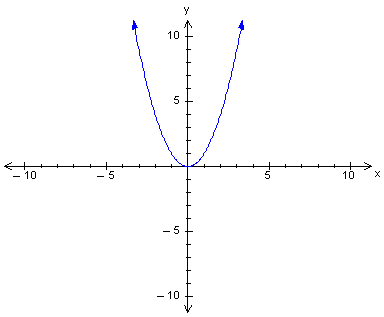
In mathematics, one often encounters curves, often as graphs of functions. In the two-dimensional case, these graphs often come about when a dependent variable y has some relationship with an independent variable x, e.g. the parabola y = x².



The graph of the function y = x² is a pictorial representation of this specific relationship between y and x.

Alternatively, we may encounter some more complicated graphs when we allow both x and y to be dependent variables of another variable t, called a parameter. For example, consider the parametric function defined by the two equations y = t² and
x = t, where we specify that the independent variable t can take any real number value. To graph this function on an xy-plane like before, we find the ordered pair (x,y) for each value of t and graph these points.

The perceptive reader will have noted that, through a simple substitution, the two equations of the parametric function above can be combined into the simple relation
y = x², the same parabola as before. Thus the graph of our parametric function is precisely the same as that of our original function, and they represent the same curve in the xy-plane. We say that the parabola is parametrized by y = t², x = t, -∞ < t < +∞, where the inequality specifies the domain of t.

However, though some parametric functions can be easily expressed simply with x and y alone, others do not create a simple, or even single-valued, dependence. Consider the more complicated parametric function y = 3cos(3t) + t, x = sin(t), and its graph in the xy-plane, below (for convenience, t is restricted to the domain -2π/3 < t < 2π on the graph below):



In such a function, substituting to obtain a relation directly between y and x would be much more complicated, and could not be a function of the form y = f(x) anyway as some values of x correspond to multiple values of y. Such curves can also intersect themselves many times, as the one above demonstrates.

Yet another way to look at a parametric function is as a mapping from 1-dimensional space (the "number line" of t) to 2-dimensional space (the xy-plane). In fact, we shall define the term curve as the range in 2-dimensional Euclidean space of such a mapping. We also specify that this mapping must be continuous, i.e. that the graph of the curve does not have any "jumps".

From now on we shall consider only mappings of the unit interval, therefore setting 0 ≤ t ≤ 1. The intuitive idea of the range, or image, of this type of curve in the xy-plane is that it is very "narrow", and does not have any area. For example, for any rectangle in the plane, one can easily measure area, but the area of just one of the sides is zero, or for that matter, the area of all four sides (for more about areas, see here). Only the region contained by the four sides has positive area.

However, in 1890, the Italian mathematician Giuseppe Peano made a remarkable discovery. There is a curve whose domain is the unit interval and whose image (graph) fills the entire unit square! (in the xy-plane, this is defined as the region such that both 0 ≤ x ≤ 1 and 0 ≤ y ≤ 1 are satisfied) In other words, a single line can take up a square, even one mapped from a finite interval.

It is crucial to note the significance of the fact that the mapping is continuous, i.e. produces a curve that fills the unit square. It is relatively "easy" to create a mapping from the unit interval to the unit square without this restriction. One way is through use of a number's decimal expansion (in base 10 notation).

Any number in the unit interval can be written in the form 0.a₁a₂a₃..., where we use 0.999... to obtain 1. Consider the function f defined on the unit interval, that "splits" the decimal expansion into two parts and makes each of these a coordinate of a point in the unit square, with

f(0.a₁a₂a₃a₄a₅a₆...) = (0.a₁a₃a₅,0.a₂a₄a₆...).

To ensure that this function is well-defined, we must "make up our minds" what decimal expansion to use to represent numbers such as 1/2, which equals both 0.5000... and 0.4999.... To remedy this, simply chose as the input of the function the terminating (where terminating means that for some N, n > N implies a_n = 0; for the terminating decimal expansion of 1/2, set N ≡ 1) expansion. Thus f(1/2) ≡ f(0.5000...) and not f(0.4999...). The diagram below indicates graphically the domain and range of the mapping, along with its effect on a selected point.



The function f defined on the unit interval in t-space has as its range the entire unit square in the xy-plane. To see that the entire square is filled, let (0.a₁a₂a₃...,0.b₁b₂b₃...) be a point of the unit square. Then it is easily seen that 0.a₁b₁a₂b₂a₃b₃... maps to this point under f. Since every point in the unit square can be expressed this way, the mapping fills it in its entirety, confirming that the unit interval has "just as many" points as the unit square.

But is the mapping above continuous? It turns out that it is not. For a proof of this fact, and an example of a space-filling curve (where continuity is required), see the next post.

Sources: Counterexamples in Analysis by Bernard R. Gelbaum and John M. H. Olmsted, Space-filling Curve on Wikipedia

Milankovitch Cycles 3

This is the third part of a series on the celestial cycles that periodically influence Earth's climate. For the first part, see here. For the second, see here.

In the first two parts of this post, two types of precession and their combined effect on the Earth's climate were explored. However, the Earth's orbit, as well as rotating over time, also varies in eccentricity. Currently, the eccentricity of Earth's orbit is about 0.017. However, due to slight perturbations from the other planets, the elongation of the ellipse that is Earth's orbit changes over time, going as low as 0.005 (nearly a perfect circle) and as high as 0.058. The mean value of the cycle is 0.028.

Unlike the variations discussed thus far, eccentricity variation does not have a simple cycle, but is rather a sum of component cycles, with all of the planets adding a contribution, some greater than others. Since these components are of different periods, simply evaluating the period by multiplying yields an exact period longer than the age of the Solar System. Thus one must use an "approximate" period that yields a cyclic variation, but within a certain error margin. Such a approximation yields a period of about 100,000 years, but with error margins that vary considerably.



The above diagram is an analysis of the periods of the eccentricity variations in the Earth's orbit. The x-axis has lengths of periods in thousands of years, organized logarithmically. For example, the value of 3 on the x-axis corresponds to a period of 2³*1000 = 8000 years. The y-axis indicates "how closely" the eccentricity variation has a component with a period of a given length. For example, as indicated, there is a peak in the curve labeled "413", meaning that it occurs at 413,000 years. The peak indicates that there is a significant component of the variation with a period of this length.

Overall, the eccentricity variation has the effect of accentuating or dampening the effects of axial and apsidal precession. Before we delve into the climatological effects more fully, one more variation must be considered: axial tilt variation.

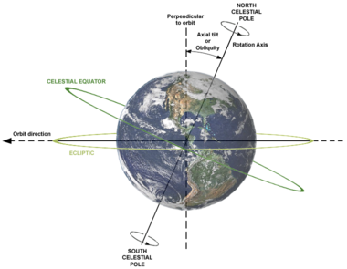
In addition, to the Earth's axis precessing in a circular motion, the obliquity of the axis, or the angle between the line through the center of the Earth perpendicular to the plane of the Earth's orbit and the line of the Earth's poles, changes in an approximately periodic manner. This process is also called nutation.



A diagram illustrating the obliquity of the Earth's axis. However, the tilt shown in the figure, which is currently about 23.4°, is not constant. It too changes with time, with a period of about 41,000 years, varying from 22.1° to 24.5° over its cycle.



The image shows the highest and lowest obliquities that Earth's axis experiences during its cycle. The current obliquity is near the midpoint of the two end values and is decreasing towards 22.1°. However, the amplitude of the variation of the obliquity over its period is not constant. The high and low values shown in the above diagram represent the most extreme variation, but some 41,000 year periods have seen variation of less than half a degree.

The Moon, which exerts gravitational forces on the Earth, acts to stabilize the variation in the position of the Earth's axis. It has been estimated that, without the Moon, the Earth's obliquity could vary enormously, on the scale of tens of degrees over its period. The influence that the Moon has on stabilizing the Earth's axis is quite important in keeping climate patterns stable. Without it, the Earth's climate could vary chaotically, with formerly polar regions becoming tropical and vice versa within tens of thousands of years which, though still a long period, would be devastating to delicate ecosystems and biodiversity.

Both of these variations have great effects on climate, the most significant of which are the amplitudes of seasonal variation. Near the highest eccentricity over the period of variation in its orbit, the Earth receives over 20% more sunlight (per unit area) at perihelion than aphelion. Due to the dampening effect of the insulation of Earth's atmosphere, the planet's heat content does not vary to this degree. However, seasonal variation would increase significantly, making these phases of the eccentricity cycle more susceptible to ice ages, as is reflected in paleoclimatological records.

Thus far, we have been treating the properties of the orbit of the Earth and all its effects on climate as if it were lying exactly in the plane of the Solar System. However, the orbit is also inclined from the plane, and this inclination varies. Before discussing the climatological effects of this variance, we must pin down precisely what the "plane of the Solar System" is.

On Earth, we typically consider the positions of bodies in the sky relative to the plane of the ecliptic, which is the plane of Earth's orbit (the ecliptic itself is the "intersection" of this plane with the celestial sphere). However, abandoning this geocentric view, we consider what is called the invariable plane. To find the invariable plane, one must find the barycenter, or center of mass, of the Solar System. The Solar System as a whole (neglecting any internal interactions) behaves as if it is a single object with a mass equivalent to that of the Solar System at its barycenter. The average rotational properties of all bodies of the Solar System provide the angular momentum vector for this ersatz representation of the system, and the invariable plane is defined as the plane passing through the barycenter perpendicular to this vector.



The angular momentum vector for an object is perpendicular to the plane of rotation, as in the top above, where L is the direction of the vector. Similarly, the angular momentum of the imaginary object representing the Solar System is perpendicular to its (again imaginary) plane of rotation.

The Sun, being on top of the center of gravity of the Solar System, does not contribute significantly to its overall angular momentum. The biggest contributions come from the gas giants, particularly Jupiter. The angle between the plane of Earth's orbit and this invariable plane is about 1.57°, which varies with a period of about 100,000 years. The places where the Earth's orbit crosses the invariable plane "going up" and "going down" are called the ascending node and descending node, respectively, and these presently occur on July 9 and January 9, respectively. Note that these nodes can be defined with respect to any plane, but we are taking it to be the invariable plane in this instance.



The above figure is a summary of some other orbital parameters of a celestial body, including the ascending and descending nodes and their longitudes, i.e., their angle from a reference direction in the invariable plane. The inclination of Earth's orbit and the position of these nodes have subtle and varied effects on climate; the positions of the nodes effect where the Earth passes through meteor showers. These, in turn, create atmospheric dust, especially in the polar regions, that form high-altitude clouds, as water vapor clings to the dust particles. These clouds are called noctilucent clouds, and a possible correlation between their abundance and ice ages has been observed in geologic records.

Milankovitch cycles help to explain at least some of the cycles of cooling and warming that the Earth experiences. However, some important disclaimers must be made. First, some feedback mechanisms help to accentuate or dampen any climatological changes brought about by orbital or rotational properties. For example, in a warming period, the polar ice caps shrink, releasing some trapped carbon dioxide that causes further warming. Therefore, even changes that are started by the Milankovitch cycles cannot be solely attributed to the cosmos, as they are but the beginning of a chain reaction here on Earth.

Second, there are many climage changes that cannot be explained through Milankovitch cycles. Large meteoroid impacts, volcanic eruptions, and other Earth-based phenomena could change or even counteract any effect of the orbit on Earth's climate, and often work in much shorter time periods.

Despite these shortcomings, the Milankovitch cycles have explained much about past climate variation on Earth, and may play a significant role in the future. The complicated web of cause and effect between the cycles and various periods of Earth's geologic history is not yet fully elucidated, but many significant correlations have been observed that promise to help us understand our planet's history.

Sources: Milankovitch Cycles on Wikipedia, http://www.clim-past-discuss.net/2/519/2006/cpd-2-519-2006.pdf,http://bugle.imcce.fr/fr/presentation/equipes/ASD/person/Laskar/misc_files/Laskar_Robutel_1993.pdf

Milankovitch Cycles 2

This is the second part of a series on the celestial cycles that periodically influence Earth's climate. For the first part, see here.

It was discussed in the last post that Earth's orbit, though very closely approximating a conic section, rotates over time with respect to its apsides, mainly due to the gas giants. However, another type of precession must also be considered: axial procession. This precession, rather than being involved with the orbit of the Earth, is concerned with its rotation.



The Earth revolves about an axis through its center, but this axis is not exactly perpendicular to the plane of the Earth and the Sun (see the figure above). Thus, at any given time, portions of the globe receive more sunlight than others over the course of a day. The hemisphere tilted away from the Sun and receiving less solar radiation is experiencing winter, and the hemisphere tilted toward the Sun and receiving more radiation is in summer. Over a complete revolution of the Earth around the Sun, different areas of the Earth are irradiated differently. The angle of the Earth's axis from the imaginary line through the center of the Earth perpendicular to the plane of the Solar system is 23.4°.



In the process of axial precession, the tilt of the axis does not change. The direction of the axis merely follows a circle (the white circle shown in the figure) with respect to the stars. A complete cycle of the axis takes 26,000 years. As this cycle occurs, the Earth's axis will point to different stars, so the "pole stars" will change over the period. For example, the closest fairly bright star to the celestial north pole (the position among the stars found by extending the Earth's axis into space) is currently Polaris, but over the 26,000 year period, the pole will drift, and become close to other stars, notably Vega and Deneb. Axial precession is caused by forces exerted by the Sun and Moon.

In addition to alterations of the appearance of the celestial sphere, axial precession also causes changes in climate. However, while apsidal precession changes the position of the apsides along the Earth's orbit, axial precession slowly shifts the position of the equinoxes along the orbit. To be more specific, the equinoxes move "backward" relative to the revolution of the Earth. This effect leads to some different definitions of the word "year". A sidereal year is the length of time it takes for the Earth to complete a orbit with respect to the stars, and is in many ways the "simplest" way to define a year. The length of the sidereal year is 365.256 days.

But this year is not that on which our calendar is based; our calendar is based on the tropical year, or the length of a complete cycle of seasons. This is loosely equal to the time from one equinox to the next. There is a slight subtlety here, though: the equinoxes do not shift at the same rate due to the eccentricity of the Earth's orbit. Due to the inequality of the lengths of the seasons, the vernal and autumnal equinox do not precess at the same rate. The equinox closer to perihelion "moves faster" than that near aphelion. Averaging the two rates gives the value used in calculating the tropical year. The tropical year is 365.2422 days, a slightly, but meaningfully different value than the sidereal year.

Thus the equinoxes and solstices will stay at approximately the same date on our (Gregorian) calendar, since this calendar is built around the tropical year using the following rules:

1. A regular year is 365 days
2. If the year is a number divisible by 4, it is a leap year, containing 366 days
• This makes the "average" year over a 4-year period equal to 365.25 days
3. But if a year is divisible by 100, it is not a leap year
• Over the 100-year period 1900-1999, for example, there were 24 leap years: all years divisible by 4 except 1900
• This yields an "average" year of 365.24 days
4. Finally, if the year number is divisible by 400 it is a leap year
• Over the 400-year period 1700-2099, for example, there are 97 leap years: 96 years divisible by 4 but not 100, three years, namely 1700, 1800, and 1900, that were not leap years, and one year, 2000, which by the above rule was a leap year
• These rules yield an "average" year over the 400-year period of 365.2425 days

This final value for the average year is only about 0.0003 years off the actual value of the tropical year, equal to an error of about 158 minutes per 400 years. There have been proposals to correct this small error by perhaps making the year 4000 not a leap year, but no such proposal has been passed.

Returning to the effect of axial precession on the climate, it has an essentially the same effect as apsidal precession, in that both cause changes in the equinoxes relative to the Earth's orbit. These two types of precession essentially "add" yielding a period of 21,000 years. What this means is that, relative to the tropical year, which is measured by the equinoxes, the perihelion will return to the same position every 21,000 years. To obtain this figure, consider the time which it takes for an equinox to travel fully around Earth's orbit: 26,000 years. Since the tropical year is shorter than the sidereal year, the equinoxes move backward with respect to the Earth's orbit, i.e. opposite to its direction of motion. In this same time, however, perihelion will shift forward by a certain amount, reducing the time that must elapse before the two again coincide to 21,000 years. Therefore, in this time, the Northern hemisphere winter, initially coinciding with perihelion, will cycle completely, and once again coincide with perihelion at the end of the interval.

However, in addition to traveling through a cycle, the amplitude of the variations of the positions of the Earth's orbit and axis also vary, as we shall see in the next post.

Sources: Milankovitch Cycles, Axial Precession on Wikipedia

Milankovitch Cycles

Milankovitch cycles, named after Milutin Milanković, a Serbian mathematician, are the periodic changes in the Earth's orbit and rotation that are the cause of gradual climate changes over periods of tens or hundreds of thousands of years. The composition of all the separate cycles involved yields a fairly complete long-term climactic picture.

In an idealized two-body problem, in which the Earth and the Sun are point masses isolated from the rest of the masses in the Universe, and assuming the orbiting body, the Earth, to be negligible in mass in comparison with the Sun, the bodies behave very predictably. The orbit of the less massive body is a conic section, with the Sun at one of the foci. "Conic section" is the general term for circles, ellipses, parabolas, and hyperbolas, each of which is depicted below.



All of the above conic sections share a focus (the dot at the center of the figure). For a circle, there is only one focus, and it is located at the center of the circle. For all other conic sections, two foci and a additional parameter (variable) determine them uniquely.

The defining property of a conic section, the one which determines its type, is a value known as eccentricity, denoted e. The parameter e is some nonnegative real number. If e = 0, the conic section is a circle. If it is between 0 and 1, the conic section is an ellipse, with the ellipse becoming more elongated as the eccentricity increases from 0 to 1. If e is exactly 1, then the curve is a parabola, and if e > 1, it is a hyperbola. Conic sections of eccentricity less than 1 represent orbits in which the orbiting object is trapped in the gravitational field of the larger object. Such orbits are periodic, and thus repeat after some amount of time. The others, of eccentricity 1 or greater, represent paths of objects in which the gravitational attraction of the larger mass is not enough to trap the smaller object, and it escapes.

These curves represent remarkably accurate approximations to planets' actual orbits, but are slightly different due to perturbations from other planets in their system. These perturbations often cause gradual changes in the shape or position of the orbit over time. We shall now focus our attention to the Earth's orbit.

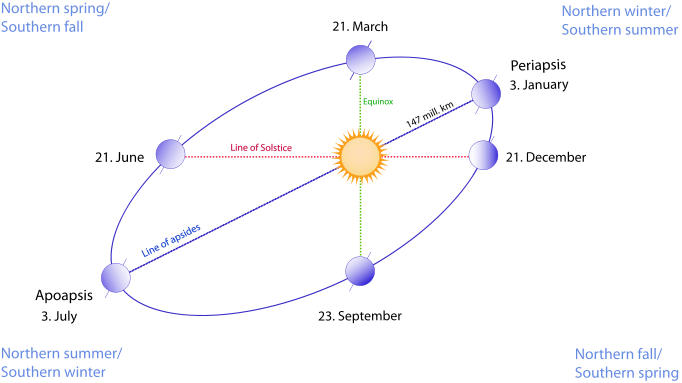
The eccentricity of the Earth's orbit is about 0.0167, meaning that the orbit of the Earth is very nearly a circle, and only slightly elliptic. However, even this slight elongation causes the Earth to be closer to the Sun in some parts of its orbit than others. Earth's closest point to the Sun is called the perihelion (or periapsis) of the orbit, and the farthest point the aphelion (or apoapsis). These extreme points are called the apsides, and are always opposite one another about the focus.



In the case of the Earth, the difference between aphelion and perihelion is about 3 million miles, or 5 million kilometers, which is not too large relative to its average distance from the Sun of 93 million miles. Despite this, the eccentricity of the Earth's orbit greatly affects our climate. Currently, perihelion occurs during January and aphelion during July, as shown above (the eccentricity is exaggerated for emphasis). However, due to the gravitational influences of the other planets, particularly Jupiter and Saturn, the apsides precess about Earth's orbit. This cycle, called the cycle of apsidal precession, takes place relative to a fixed direction, called the reference direction.



The above figure illustrates apsidal procession, with both eccentricity and rate of precession exaggerated. If we treat the apsidal line of the first orbit (the horizontal line in the figure) as the reference direction, the angle (in the positive counterclockwise sense) that the apsidal line of each subsequent orbit (on the periapsal side) is what is called the angle of periapsis. Over a full cycle of apsidal procession, the angle of periapsis increases by 360°, i.e., the orbit returns to its former position. For the Earth, this cycle takes 112,000 years. This is one of the Milankovitch cycles, and it has a profound impact on our climate.

For the northern hemisphere, perihelion occurs during winter, and aphelion during summer. Since the Earth receives 6.8% more sunlight at perihelion (this figure comes from the fact that the light intensity dies off with squared distance; even though the distance of the Earth at aphelion is only 103.4% of that at perihelion, the light intensity differs by about 6.8%), our planet actually receives more sunlight in northern hemisphere winter than summer. However, the Earth's axial tilt, which we will consider later, dominates this relatively small effect. Currently, apsidal procession slightly dampens the seasonal variations in climate in the northern hemisphere, while accentuating them in the southern hemisphere.

If apsidal procession were the only cause of climactic variance, the state of the northern and southern hemispheres (with respect to the dampening or accentuating of seasonal variances) would reverse in 56,000 years, but apsidal precession is not the only effect on the seasons (see the next post).

One final interesting effect that the apsides have on our seasons is their lengths. The Earth travels slightly faster at perihelion, as it is closer to the Sun, so whatever season the Earth is experiencing at perihelion will be slightly shorter than the opposite season at aphelion, where the Earth is moving at its slowest relative to the Sun. Thus northern hemisphere winter (the time between the winter solstice and vernal equinox) is over four days shorter than summer. Through apsidal precession other seasons will become the longest over the 112,000 year time period.

Sources: Milankovitch Cycles on Wikipedia, http://www.jimloy.com/geometry/conic0.htm, http://huminities.blogspot.com/, http://www.answers.com/topic/why-are-the-lengths-of-the-seasons-not-equal

2013 Season Summary

The 2013 Atlantic hurricane season was below average, with

15 cyclones attaining tropical depression status,
14 cyclones attaining tropical storm status,
2 cyclones attaining hurricane status, and
0 cyclones attaining major hurricane status.

Before the beginning of the season I predicted that there would be

18 cyclones attaining tropical depression status,
16 cyclones attaining tropical storm status,
9 cyclones attaining hurricane status, and
4 cyclones attaining major hurricane status.

My predictions were well above the actual number of tropical cyclones in all categories, but particularly in the "hurricanes" and "major hurricanes" categories.

The ENSO was roughly neutral this year, with neither a significant El Nino nor a notable La Nina event occurring. Due to the lack of an El Nino, upper-level winds were favorable for tropical cyclone formation. In addition, ocean temperatures throughout the tropical Atlantic were warm (though they were relatively cold in the Gulf of Mexico for parts of the season). However, other, unforeseen conditions overwhelmed these favorable factors. During early August, an exceptionally large volume of dust moved off of the Saharan desert into the eastern Atlantic. This dust blocked some of the sunlight that would otherwise each the ocean surface, cooling water temperatures and inhibiting thunderstorm formation. This event prevented cyclone formation through the first half of August, a normally active period.

In addition, cyclones were plagued by large areas of stable air throughout the season, particularly in the central Atlantic. To survive, tropical cyclones require continued updrafts of warm and humid air to fuel convective growth. This is known as unstable air. Stable air, on the other hand, can be deadly to tropical cyclones. Dorian and Humberto in particular both met their swift demise due to stable air masses. Finally, wind shear was anomalously strong given the neutral ENSO, particularly over the Gulf of Mexico. For example, Tropical Storm Karen moved into the Gulf as a tropical storm in early October. Typically, such a storm would present a great danger to some landmass, and certainly make landfall, but Karen did neither, as shear destroyed the system before it reached the U.S. coastline.

Some notable facts and statistics concerning the 2013 season are:

• The name Ingrid was retired after the season's conclusion due to the damage Hurricane Ingrid caused in Mexico
• Tropical Storm Andrea was the only cyclone of the season to make landfall in the U.S., and it did so with 65 mph winds
• No cyclones made landfall at hurricane intensity during the season
• The only hurricanes during the season where Humberto and Ingrid; the last time only two hurricanes formed was 1982
• There were no major hurricanes for the first time since 1994
• The season's strongest storm was Hurricane Humberto, which had maximum winds of 85 mph and a minimum pressure of 980 mb; this is the first time no cyclone reached category 2 intensity since 1968
• The ACE of the season was 33.4, the lowest since 1994
• An unnamed subtropical storm formed in the Atlantic basin on December 4, unnamed because it was not recognized as such at the time, but only during post-season analysis; it was the first December storm since 2007

Overall, the 2013 season was unexpectedly quiet, and caused little damage in comparison to other seasons in recent years.

Tropical Storm Melissa (2013)

Storm Active: November 18-22

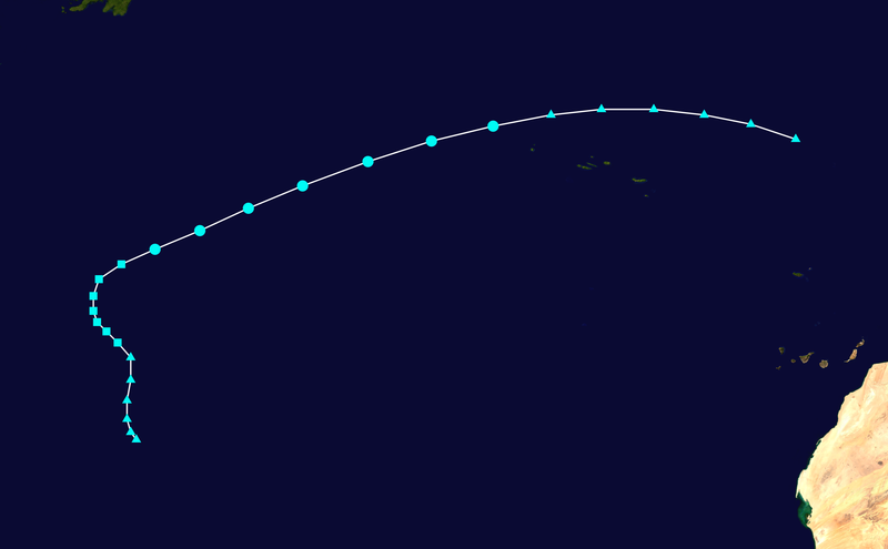
On November 12, a very strong cold front swept southeastward over the eastern half of the United States, bringing cold air in its wake as it departed the coast. A few days later, the large frontal boundary became stationary over the central Atlantic. By November 16, a broad area of low pressure was forming along the southern edge of the front, which at that time lay well northeast of Puerto Rico. The low had become better defined and produced winds of gale force on November 17. Meanwhile, the system was moving north-northwestward and developing more concentrated convection. By November 18, the low was deepening rapidly and a prominent banding feature beginning in the western side of the circulation and wrapping clockwise to its southeastern edge appeared. The frontal boundary that had been associated with the low was gone by that afternoon, so the system was designated Subtropical Storm Melissa.

Melissa was subtropical due to its broad wind field and circulation, but it was already a strong cyclone, and strengthened steadily into the morning of November 19 as it moved northwestward. During the afternoon, a cold front approaching from the west caused the cyclone to turn northeastward and begin to accelerate as Melissa reached its peak intensity as a subtropical storm of 65 mph winds and a pressure of 982 mb. Though convection became a little closer to the center of Melissa that evening, the outflow of the system had grown less impressive, and the maximum winds diminished through the early morning of November 20.

Later that morning, however, better defined curved bands developed, and enough convection appeared near the center that it was clear that the system had made the transition to Tropical Storm Melissa. Over the next day, the cyclone continued to move quickly to the northeast and then east-northeast into cooler water, but still managed to maintain tropical cyclone status into November 21. That afternoon, Melissa's peak winds actually increased to 65 mph once again, with a pressure of 980 mb. Since the system was over very cold water at the time, the strengthening indicated that Melissa would very soon be post-tropical. In fact, the remaining banding features continued to deteriorate that evening, and Melissa became post-tropical.

By this time, the cyclone had passed just north of the Azores. The outer wind field of the system caused gusty winds in the islands, but the diminishing convection was such that no significant rainfall occurred. The system that had been Melissa continued roughly eastward until its dissipation.

The above image shows Melissa as a subtropical storm on November 19. At this time, the center was still mainly devoid of convection, a common feature of subtropical storms.

Melissa did not significantly affect any land mass during its lifetime.

Tropical Storm Lorenzo (2013)

Storm Active: October 21-24

On October 20, a low pressure center formed along a trough over the central Atlantic ocean and thunderstorms began to concentrate about it. By the next day, a surface circulation was developing, and the system was designated Tropical Depression Thirteen that evening. The cyclone was already moving northeastward at the time of formation, and continued to move out into the open waters of the Atlantic.

Overnight and into the morning of October 22, Thirteen became more organized as convection continued to increase in the relatively friendly atmospheric environment. Soon, the cyclone had developed a symmetric dense overcast, and thus strengthened into Tropical Storm Lorenzo. The storm's organization increased further that morning, bringing Lorenzo to its peak intensity of 50 mph winds and a pressure of 1003 mb. By this time, the system was moving toward the east, having navigated around the upper edge of a mid-level ridge.

Lorenzo maintained its intensity until October 23, when shear increased substantially out of the northwest and decoupled the surface and mid-level circulations of the system and displaced convection from the cyclone's eastern side. Before long, all thunderstorm activity had been obliterated by the blast of wind shear, and Lorenzo was downgraded to a tropical depression that night. During the morning of October 24, the system degenerated into a remnant low. The low dissipated a few days later.

The above image shows Lorenzo near its peak intensity.

Lorenzo was a short-lived tropical storm, and did not affect land.

Tropical Storm Karen (2013)

Storm Active: October 3-6

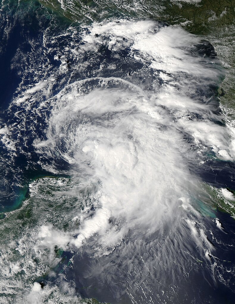
On September 28, a tropical disturbance formed in the southern Caribbean sea, and began to track slowly northwestward. Over the next couple of days, the trough associated with the disturbance became much better defined, but the convection associated with the system remained disorganized. Convection increased markedly around the deepening low pressure center during the days of October 1 and 2 as the system approached the Gulf of Mexico, but aircraft investigation did not discover a well-defined center of circulation. The system caused very heavy rainfall and gusty winds in eastern Cuba as it passed by, and on October 3, as the system entered the southeastern Gulf of Mexico, a defined center appeared. The system was upgraded to Tropical Storm Karen. Due to the exceptionally high winds found east of the center, the initial intensity of the cyclone was already 60 mph!

Though by the measured wind speeds, Karen was a strong tropical storm, it did not appear as such. Strong upper-level winds constantly exposed the center overnight and into October 4 as the storm moved into the central Gulf. Over the next day, Karen continued to struggle north-northwestward, weakening gradually as wind shear displaced thunderstorm activity to the east of the center. By the morning of October 5, the system had become a minimal tropical storm and was approaching the Gulf Coast.

Later that day, Karen paused again, becoming nearly stationary south of the Louisiana coastline due to a ridge situated to its east. Atmospheric conditions continued to worsen that evening, and it became evident that the cyclone's circulation was slowly deteriorating. It was downgraded to a tropical depression overnight, and dissipated early on September 6, never having made landfall. Some of the moisture associated with Karen moved northward along a frontal boundary over the next day and caused enhanced rainfall up and down the east coast.

Even at peak intensity, when the cyclone was producing 65 mph winds, Karen did not exhibit much convective organization.

Probably due to its shallow circulation, Karen's forward motion diminished as it entered the northern Gulf of Mexico and the system was ripped apart by wind shear.