Behavior of the Gamma Function

In the previous post, the idea of the Gamma function, or the extension of the factorial beyond the positive integers, was introduced. In addition, an expression for it, in the form of an infinite product, was discussed. But how does the function actually behave outside of the integers? First, we shall consider some basic facts:

We have already confirmed that the factorial function grows faster than the polynomial and exponential functions. In addition, it grows slower than the function x^x, a fact which can be confirmed without difficulty in a similar manner.

Also of importance is the total determination of the function on the real numbers given only its value on the interval (0,1) (the real numbers from 0 to 1 not including 0 or 1). This is due to one of the two fundamental properties of the Gamma function: Γ(x + 1) = xΓ(x). Since any real number can be expressed as the sum of an integer and a number between zero and one, iterated applications of the above property will yield the desired value. For example,

Γ(3.5) = (2.5)Γ(2.5) = (2.5)(1.5)Γ(1.5) = (2.5)(1.5)(0.5)Γ(0.5), thus reducing the problem of calculating the value of the function over the real numbers to that of calculating it only between zero and one.

Of the values on (0,1), all can be approximated numerically to any degree of accuracy with the infinite product, but only one, Γ(1/2), is known in closed form. Its exact value is

Γ(1/2) = (π)^1/2, a fact that was discovered when a previously known infinite product that equaled π was identified with the expression when 1/2 is substituted in for the definition of Γ(x). Thus, any real number with fractional part 1/2 can be expressed in closed form. The graph of the Gamma function on the real line is as shown below.



It is clear that the Gamma function is undefined at each non-positive integer, as is consistent with the definition. In addition, there is no number x such that Γ(x) = 0. The graph alternates between positive and negative on the intervals between the negative integers because going from one interval to the next is equivalent to multiplying (or dividing) by a negative number in accordance with the above rule.

However, the Gamma function is not even limited to the real line. It is also defined for all complex values using the same infinite product as before. The product is defined at all complex numbers off the real line, i.e. there are no additional discontinuities beyond the non-positive integers. The behavior of the Gamma function over the entire complex plane is illustrated below.

To graph such a function on the complex plane would normally require four axes, two for the input z, the real part and the imaginary part, and two for the output Γ(z). Since there are only two dimensions available when graphing on a plane, hue and lightness are used in addition to illustrate the behavior of the function. The two physical dimensions of the graph illustrate the position of the input on the complex plane in accordance with the numbered axes (horizontal: real axis, vertical: imaginary axis). The output is colored according to the scheme illustrated below:

The modulus of the complex number is indicated by its lightness; numbers closer to zero are indicated by darker colors, while complex numbers far from zero are whiter. Furthermore, the argument, or angle made with the positive horizontal axis, is indicated by hue. For example, a complex number with an argument near zero appears red, while one with an argument near π (180°) is blue. Returning to the complex "graph" of the Gamma Function, it is easy to see how the graph on the real line is a cross section of the full graph: along the horizontal real axis in the middle, the output is red (positive real number, argument 0) for positive input, and alternating between red and light blue (negative real number, argument π) for negative integers. Also, as one travels further negative, the outputs become very small (darker), except for the spike at each negative integer where the function goes to infinity (white dots). The points at which the Gamma function is undefined are called poles.

Over the rest of the complex plane, it can be seen that the function's value at any complex number is the conjugate (reflection over the real axis) of the value at its conjugate. In other words, the output at two points that are reflections over the real axis have the "opposite" colors indicated by the scheme above. In equation form,

All of these properties are illustrated on a copy of the complex graph above:

Due to its nature as an extension of the factorials, the Gamma function allows an analogous broadening of the field of probability theory. It also finds applications related to binomials and the evaluation of coefficients in a product. Finally, it is related to other functions involved in number theory, and emerges in computations in a variety of mathematical fields.

---

Sources: Gamma Function, Wikipedia, Mathematical Thought from Ancient to Modern Times (Vol. 2) by Morris Kline

The Gamma Function

The concept of the "factorial" function in mathematics is well-known. For any positive integer n, n factorial, denoted n!, is the product of n with all smaller positive integers. In equation form,

n! = (n)*(n-1)*(n-2)*...*3*2*1

The first few values are 1! = 1, 2! = 2*1 = 2, 3! = 3*2*1 = 6, 4! = 4*3*2*1 = 24,... In addition, one can easily see that dividing the factorial of a number by the number itself yields the previous factorial, that is, n!/n = (n-1)!. As an example, 4!/4 = 24/4 = 6 = 3!. Extrapolating backward, 1!/1 = 1 would be the value of zero factorial. Thus we consider 0! = 1.

The problem with which we are concerned is how to extend the idea of factorials to values other than the positive integers, a procedure called interpolation. In other words, we seek a function, f(x) that generates the factorials for the positive integers but also is defined on non-integers.

First to be considered are the polynomial and exponential functions, i.e. those of the form xⁿ and a^x, respectively, for natural numbers n and general positive numbers a, where x is the variable quantity. Can either of these types, or additions/subtractions thereof, yield a function that matches the factorials? The answer is no, for the following reason: the factorial function grows faster than any polynomial or exponential function. This means that if one increases x high enough, x! (assuming x is an integer) will always exceed a function of the above types. To see this, we shall examine the growth of polynomial and exponential functions in turn.

For any function xⁿ, xⁿ exceeds x! at x = n, as nⁿ is a product of n n's, while n! is a product of n numbers less than or equal to n. However, consider the comparison of values at x = n²:

(n²)ⁿ = n²ⁿ, while
(n²)! = n²*(n²-1)*...*n*...*2*1.

A close examination of the expansion of the factorial allows one to see that there are n² - n terms exceeding n (those that occur prior to n), while the polynomial value is a product with 2n terms, all equaling n. So as long as
n² - n > 2n, the factorial will be greater. This is true for all n > 3. Also, for any xⁿ, the ratio of the value of this function at x = a + 1 to that at a for positive integral a approaches 1 as a increases, as this ratio is

Since (a + 1)/a clearly approaches 1 as a increases, so does this quantity taken to a constant positive power. In contrast, the ratio (a + 1)!/a! always equals a + 1, and this continues to increase as a increases. Thus, once a factorial exceeds a polynomial, its exceptionally large rate of change insures that it stays above the polynomial. To treat the cases where n = 2,3 and n² - n ≤ 2n, it is easy to see that any polynomial with an x⁴ term exceeds one with either an x² or an x³ as its highest term, and since the factorial exceeds x⁴, it is also greater than the other two.

For exponential functions, it suffices to treat those a^x where a is an integer. If the factorial exceeds these, it also exceeds any exponential function for real a. Going as before, at x = a, a^x is greater than a! for the same reasons as for the polynomials. However, each increase of x by 1 beyond this is equivalent to multiplying the exponential function by a, but the factorial by a number greater than a:
a^{a + 1} = a*a^a, while (a + 1)! = (a + 1)*a! and so on. The factorial clearly increases faster, and thus "catches up with" and exceeds the exponential function. To further illustrate this, consider the graph below (click to enlarge):



The polynomial function x¹⁰ (green), the exponential function 10^x (red), and the factorial function x! (blue) compared on a logarithmic graph. The factorial function is interpolated here, but for the time being, we still consider only integer values. Initially, when x is between 2 and 10, the polynomial is the greatest. At 10, the polynomial and exponential functions are obviously equal. Finally, x = 25 is the first point at which the factorial exceeds both functions, the value of 25! being over ten trillion trillion!

The factorial, however, can be shown to increase less rapidly than functions such as x^x. In fact, no combination of elementary functions can represent the factorial. To find an expression for the factorial, one must consider more precisely the conditions that must be met. There are an infinite number of curves through any set of points, and therefore the condition that the function coincide with the factorial for positive integers is insufficient to define it uniquely. Therefore, the following two conditions are given for the function f:

f(0) = 1, and
f(x + 1) = (x + 1)f(x).

The second condition generalizes the standard rule for factorials, (n + 1)! =
(n + 1)n!, to any x.

The function that satisfies these conditions is the Gamma function, denoted Γ(x). However, the Gamma function is actually slightly different from the factorial function, as it is translated one unit. What this means is that, for positive integers n,
Γ(n) = (n - 1)!. Therefore, the Gamma function actually satisfies

Γ(1) = 1, and
Γ(x + 1) = xΓ(x)

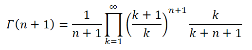
for all x. There are several ways to actually formulate the Gamma function, one being an infinite product:



In evaluating this product, the expression after the Π must be calculated for every positive integer k. Then, all of these values must be multiplied. As the upper bound on k increases to infinity, the product converges to the actual value of n!. Note that the above product is defined for every n, except for negative integers. This is because, if n is a negative integer, in the term k = -n, the denominator of k/(k + n) becomes zero. Since once term is undefined, the whole product is. In addition, due to the 1/n term outside of the infinite product, Γ(0) is undefined. Thus the Gamma function is defined for all numbers except the nonpositive integers.

Next, we must confirm that the Gamma function satisfies the required conditions, in order to see that it truly is an extension of the factorial function. It is clear that Γ(1) = 1, because, in this case, ((k + 1)/k)ⁿ = (k + 1)/k, and k/(k + n) = k/(k + 1), which is precisely the reciprocal of the first term. When these are multiplied, they yield 1, no matter the value of k. Thus the infinite product takes the form (1/1)(1*1*1*...) = 1, as desired. Next, it must be proven that Γ(n + 1) = nΓ(n). When n + 1 is substituted for n in the above product, it yields the following expression:
(1)
After some manipulation, this becomes
, (2)
as an infinite product of two terms multiplied together is the product of the infinite products of each term. The first of the two expressions in parentheses is simply the expression for Γ(n), and the value of the second can be inferred from its expansion:
(3)
The fraction (n + 1)/(n + 2) in the first term (k = 1) of the expansion is canceled by its reciprocal, which appears later as the value of (k + 1)/k when k = n + 1. Whenever the first and second fractions of the infinite product can assume reciprocal values for a positive integer value of k, they cancel, for any (k + 1)/k can be cancelled by some expression of the form (k + n)/(k + n + 1) as long as k > n. Therefore, with all of these canceled, all that remains is a product of the fractions (k + 1)/k, as k ranges from 1 to n, or, in numerical form, (2/1)*(3/2)*...*((n + 1)/n). The value of this is (n + 1)/1 = n + 1, since every other number appears once in the numerator of a term, and once in the denominator. Finally, the n + 1 that results cancels with the fraction before the second infinite product in (2), yielding simply n. Thus, finally,

Γ(n + 1) = nΓ(n),

and the infinite product formula agrees with the (shifted) factorial function for all positive integers n. The actual behavior of the Gamma function and its values are discussed in another post.

---

Sources: Gamma Function, Wikipedia, Mathematical Thought from Ancient to Modern Times, vol. 2 by Morris Kline

2012 Season Summary

The 2012 Atlantic hurricane season was above average, with

19 cyclones attaining tropical depression status
19 cyclones attaining tropical storm status
10 cyclones attaining hurricane status
1 cyclones attaining major hurricane status

Before the beginning of the season I predicted that there would be

15 cyclones attaining tropical depression status
13 cyclones attaining tropical storm status
5 cyclones attaining hurricane status
3 cyclones attaining major hurricane status

The number of tropical depressions, tropical storms, and hurricanes was well above my predictions prior to the start of the season, though there was only 1 major hurricane relative to the 3 I predicted.

Much of the discrepancy in the forecast can be explained by the status of the El Nino over the course of the season. Early in 2012, the NOAA predicted the development of a moderate El Nino event by midyear, which was to inhibit the development of cyclones in the latter half of the season. However, the development of the El Nino was delayed and inconsistent, allowing for periods of explosive cyclonic formation.

In spite of the very large number of cyclones, there was only a single major hurricane, Michael, during the season. Broader cyclones such as Ernesto, Isaac, and Leslie struggled mightily in strengthening and grossly underperformed in intensity relative to short-term forecasts. Leslie, for example, was predicted to reach strong Category 2 strength, but its peak intensity was only as a minimal Category 1. Smaller cyclones, though, did the opposite, often surviving or intensifying more than expected. Michael, the strongest cyclone by winds during the season, intensified in an only marginal environment, even doing so in relatively close proximity to the much larger Hurricane Leslie. These data are indicative of the prevalence of dry air throughout the basin during the season and also of differences in the direction of upper- and lower-level winds over the season.

Another interesting trend that emerged around early September was the development of unusual blocking patterns and lack of steering currents over the northern part of the Atlantic basin. This was due to an anomalous shift of the jet stream to the north over the Atlantic, as this allowed subtropical ridges to remain in place, and prevented cyclones from being caught in the flow of troughs, which followed a more poleward path. The trend became evident with Leslie and Michael, and was exemplified by Nadine, which survived for a very long time over the north Atlantic, and finally by Hurricane Sandy, which was able to recurve westward due to the unusual shape of the jet stream.

Some notable cyclones and facts about the season include:

• 2012 was the third Atlantic hurricane season in which two preseason storms (in this case Alberto and Beryl) formed, after 1887 and 1908
• Beryl was also the strongest Atlantic preseason cyclone since 1972
• Debby, becoming a named storm on June 23, surpassed the previous record for earliest fourth tropical cyclone formation of July 7 set during the 2005 Atlantic Hurricane Season
• Though Gordon developed into a tropical storm before Helene, the tropical depression that became Helene formed before that which became Gordon, and thus the names are reversed on the chronological listing
• Michael was the strongest storm of the season by wind speed, achieving 115 mph winds, or minimal Category 3 intensity, the lowest highest wind speed for an Atlantic hurricane season since 1994
• Hurricane Nadine spent 21.75 days as a tropical cyclone meandering around the northeast Atlantic, making it fifth on the all-time list of longest lasting tropical cyclones
• Hurricane Sandy recorded the season's minimum pressure of 940 mb as it transitioned to an extratropical cyclone and made landfall in New Jersey
• The 2012 season overall was tied for the third most active in terms of number of named storms

Overall, the 2012 Atlantic hurricane season was quite active, and included several hurricanes, but was not very intense. Hurricane landfalls included Ernesto in the Yucatan Peninsula and Isaac in Louisiana, both of which were not particularly strong, and caused relatively little damage. The Caribbean Sea was relatively quiet, as wind shear and dry air mostly kept cyclones in the region to tropical storm intensity, with the exception of Hurricane Sandy, the most notable storm of the season. Sandy, which made landfall in Jamaica, Cuba, and the Bahamas as a hurricane, went on to develop into a hybrid system and slam into the northeast coast, causing widespread damage and unprecedented storm surge along the New Jersey and New York coastlines.

Tropical Storm Tony (2012)

Storm Active: October 22-25

A tropical wave formed in association with an area of disturbed weather accompanying an upper-level low about midway between the western coast of Africa and the Lesser Antilles on October 18. This interaction sporadically produced concentrated thunderstorm activity as it moved to the northwest over the next several days.

Atmospheric conditions improved markedly on October 21, and allowed the system to organize rapidly into Tropical Depression Nineteen on October 22. The cyclone began to curve towards the northeast later that day, as a front approached from the west. By late on October 23, convection had developed close enough to the center of circulation that the cyclone was upgraded to Tropical Storm Tony.

Despite shear from the front to its west, Tony experienced modest strengthening as it accelerated to the east-northeast, and the storm reached its peak intensity of 50 mph winds and a pressure of 1000 mb on October 24. Meanwhile, Tony was beginning to exhibit nontropical characteristics; the banding features became more linear, and the circulation elongated. The transition was very gradual, however, and the system remained a tropical storm through October 25, at which time it lost any remaining tropical characteristics and was downgraded to a remnant low.



Tony as a moderate tropical storm moving rapidly to the northeast over the Central Atlantic.



Track of Tony.

Hurricane Sandy (2012)

Storm Active: October 22-29

A low pressure trough embedded in the Intertropical Convergence Zone moved into the Caribbean sea on October 18, and began to increase in shower activity the next day. On October 20, as the area of disturbed weather moved west, the pressures in the area dropped precipitously, and the circulation became much better organized.

Deep convection did not consistently accompany the system on October 21, but conditions continued to be favorable as the disturbance moved southwest, bringing some showers to Jamaica and neighboring areas. By October 22, a swirl was evident amid the clouds, and the low was classified as Tropical Depression Eighteen. The system drifted southward and organized further later that day, and strengthened into Tropical Storm Sandy.

Sandy adopted a slow but accelerating northward motion early on October 23, as a front lifted out of the northwestern Caribbean. Meanwhile, convection steadily increased with the system, and became closer to the center by later that day, causing steady strengthening. In the evening, the cloud tops of Sandy's central dense overcast cooled considerably, and the first hints of an eye feature appeared, indicating that the cyclone was undergoing rapid strengthening. Meanwhile, the outflow had improved, with heavy rain bands sweeping across Jamaica, Hispaniola, and eastern Cuba as Sandy approached. These factors caused the cyclone to be upgraded to a hurricane later that morning.

During the afternoon, the center of Sandy passed directly over eastern Jamaica, but the land interaction did almost nothing to disrupt the circulation and the system continued strengthening, as an eye appeared on infrared as well as visible satellite imagery. Over the next twelve hours, Sandy put on a burst of extremely rapid strengthening, bringing its pressure down to a value of 954 mb. Very early on October 25, the cyclone made landfall in eastern Cuba with its peak winds of 110 mph!

Sandy weakened slightly as it moved over Cuba, but emerged over water still maintaining Category 2 intensity. The cyclone slowed down considerably and turned to the north-northwest that night as it interacted with an upper-level low. Higher shear weakened the system as it lashed the Bahamas, but the structure of the storm also underwent a transformation. Convection became displaced from the center in all but the northwestern quadrant, the windfield broadened, and the outflow became more extratropical in appearance on October 26.

However, shear declined somewhat, and thunderstorm activity more completely covered the center by early on October 27. By this time, Sandy had begun to moved towards the north-northeast, fluctuating in intensity but remaining near minimal hurricane strength.

By later that day, rain bands associated with the combination of a front stalling near the U.S. east coast and the circulation of Sandy swept across numerous states, causing tropical storm force winds in the North Carolina and heavy rain in localized areas up through Virginia. Dry air also invaded the circulation of Sandy, creating a narrow ring devoid of thunderstorm activity between the central convection and outer bands. However, this did not weaken Sandy, as the system was exhibiting some subtropical behavior.

Early on October 28, the central pressure of Sandy dropped again as the cyclone deepened further, plunging to a new low of 951 mb. Meanwhile, the cyclone accelerated to the northeast, and gale force winds expanded even further, stretching from North Carolina all the way to Bermuda, and rain bands moved further up the coast, sweeping across Pennsylvania and New Jersey.

During the night, Sandy began a highly unusual turn towards the northwest, under the influence of an exceptionally strong high pressure ridge over northeastern Canada. This ridge caused an inversion in the normal path of the jet stream, diverting it so that it doubled back on itself. The cyclone began to be drawn in by this feature, and so curved in the opposite direction that tropical cyclones typically turn.

Meanwhile, as Sandy traversed the warm waters of the Gulf Stream, it actually intensified somewhat, despite being at a fairly high latitude. In addition, the pressure continued to drop. Conditions deteriorated rapidly along the Delaware and New Jersey coastlines that afternoon as the central bands of the cyclone came onshore. Hurricane force wind gusts and storm surges in excess of 5 feet were recorded up and down the coast. Sandy accelerated rapidly that afternoon, and was losing tropical characteristics as its central band became frontal in nature. Early that evening, the system recorded its minimum pressure of 940 mb, and winds of 90 mph.

Shortly afterward, around 7:00 pm EDT, Sandy was recognized as an extratropical cyclone, and the remnants of Sandy made landfall in southern New Jersey an hour later. High wind and occasional heavy rain continued as the low crossed into Pennsylvania late that night and weakened to the equivalent of a tropical storm early on October 30. The low continued westward and weakened, still causing rain and snow in the Appalachian areas until it dissipated on October 31. The remnants still caused shower activity for another few days as they moved northeast away from the United States.

Hurricane Sandy set a new record for the largest Atlantic hurricane, with a gale diameter of 945 miles a few hours before landfall in New Jersey, and was one of the costliest in U.S. history. Sandy caused widespread damage in a large swath extending from Jamaica, through Cuba and the Bahamas, and up the east coast from North Carolina to New England.



Sandy near peak intensity near landfall in eastern Cuba.



Track of Sandy.

Hurricane Rafael (2012)

Storm Active: October 12-17

On October 5, a tropical wave emerged off of Africa, but remained weak for the next several days as it traversed the eastern Atlantic. The system gradually moved over warmer waters and increased in shower activity. By October 9, the system had a well-defined low pressure center associated with it. Shear out of the west still impacted the low, but atmospheric conditions improved over the following few days.

Rain and windy conditions began to affect the Lesser Antilles and surrounding areas during the day of October 12. At this time, the convection was becoming concentrated at the center of circulation, but was still somewhat displaced to the east. Later that day, aircraft indicated that the cyclone had developed a closed center, and was thus classified Tropical Storm Rafael. At the time of its formation, the convection was still distributed linearly along the former trough boundary, and the circulation remained slightly elongated. However, the thunderstorm activity was very vigorous; there were widespread areas of heavy squalls and tropical storm force wind gusts.

Rafael moved generally to the north-northwest over the following day, and very slowly organized, with a more defined region of cold cloud tops appearing near the center during the afternoon of October 13. This initiated a period of strengthening as the center moved closer to the Virgin Islands. The system passed close to the northeastern Caribbean islands late that night with maximum winds of 50 mph as the cyclone continued its trek north.

On October 14, Rafael took a slight turn towards the northwest as the ridge over the north-central Atlantic strengthened, slowing as it did so. By this time, the cyclone had assumed a more symmetric appearance, and on October 15, the circulation finally achieved gale force winds on all sides of the center, and was near hurricane intensity. Later that night, a flare up of very strong convection appeared at the center, prompting the upgrade of Rafael to a Category 1 hurricane.

Early on October 16, the system began to accelerate northward in the flow of a trough emerging off of the U.S. coast, and vertical shear increased. Despite the intense shear, however, outflow remained remarkably healthy in all quadrants, and Rafael strengthened further, reaching its peak intensity of 90 mph winds and a pressure of 969 mb that morning. By the evening, the cyclone was approaching Bermuda as an impressively large cyclone.

The system made its closest approach to the island that night, and continued to accelerate to the north-northeast, moving away from the island at over 25 mph. Early on October 17, Rafael's circulation assumed an extratropical appearance, with a very large area of gale force winds and bands extending many hundreds of miles from the center. However, the hurricane maintained a small amount of deep convection near the center until that afternoon, at which time is was pronounced extratropical, still producing hurricane-force winds as an extratropical low. The low continued northeast before combining with another powerful system over the north Atlantic the next day.



Rafael as a Category 1 hurricane moving north into open waters.



Track of Rafael.

Tropical Storm Patty (2012)

Storm Active: October 11-13

On October 11, a low pressure center formed at the tail end of a frontal boundary extending from the northeast Atlantic down to near Hispaniola. Disturbed weather increased near the low during the following day, as the low became disassociated with the trough to its northeast.

Over the next several days, another frontal boundary began to approach the low, causing a sharp increase in wind shear. However, the low did not get caught in the flow ahead of the front, but instead remained nearly stationary just to the northeast of the Bahamas through October 10. Despite being expected to merge with the front, the system maintained its identity, and in fact became more organized, as thunderstorm activity concentrated near the center.

By the afternoon of October 11, the low had achieved enough deep convection to be considered a tropical cyclone and so was classified Tropical Depression Sixteen. That evening, the convection increased and covered the exposed circulation, and the cyclone was therefore updated to Tropical Storm Patty. Late that night, Patty unexpectedly strengthened further, and reached its peak intensity of 45 mph winds and a pressure of 1005 mb.

On October 12, a combination of strong southwesterly upper-level winds and a northeasterly low-level flow started to pull the circulation apart. Patty weakened to a tropical depression that evening as the center once again became completely exposed. By the morning of October 13, the circulation was no longer closed, and Patty was declared a remnant low. The remnants combined with a trough of the U.S. east coast shortly afterward.



Patty as a disorganized tropical storm struggling to survive just north of the Bahamas.



Track of the short-lived Patty. Most of the positions indicate occurred when the cyclone was non-tropical (triangles), with only the tiny clump of circles accounting for Patty's time as a tropical cyclone, in which it moved little.

Tropical Storm Oscar (2012)

Storm Active: October 3-5

On September 30, a tropical wave off of the coast of Africa began to show signs of an organized circulation, though convection remained limited. The disturbance moved generally west-northwest over the following two days, and increased markedly in thunderstorm activity. The circulation remained slightly elongated into October 3, but the system was sufficiently organized to be designated Tropical Depression Fifteen.

The cyclone had internal structure issues ab initio; at its formation, convection was displaced to the east and south of the circulation, and the center featured multiple vortices that only gradually consolidated. A trough descending into the central Atlantic had displaced the Bermuda high by this time, and Fifteen began to turn northward.

Overnight, winds increased slightly, and the system was upgraded to Tropical Storm Oscar. Strong upper-level winds kept the center of the cyclone exposed all through October 4, but deep convection moved a little closer to the center, and the winds within the area of shower activity increased. This brought Oscar to its peak intensity of 50 mph winds and a pressure of 997 mb.

By October 5, the trough was encroaching on the circulation of Oscar, and the rapidly deteriorating cyclone was accelerating to the northeast. By late that morning, the cyclone's elongated circulation combined with the trough of low pressure, and the system was announced dissipated.



Oscar as a strongly sheared cyclone over the far east Atlantic.



Track of Oscar.

Hurricane Nadine (2012)

Storm Active: September 11-October 4 (21.75 days as a tropical cyclone)

On September 7, a low pressure system emerged off of the western coast of Africa. The system moved over the Cape Verde Islands the next day, bringing some periods of heavy rain and gusty winds to the islands. The low slowly gained organization, with convection becoming closer to the center over the next few days as it moved westward.

Dry air briefly hindered development somewhat on September 10, but the system became slightly better organized on September 11, meriting the designation Tropical Depression Fourteen late that morning. The system turned toward the northwest that afternoon, as a weakness developed in the ridge to its north.

A central overcast developed late that night, and the central pressure dropped, so Fourteen was upgraded to Tropical Storm Nadine. Steady strengthening occurred over the next day as convection deepened, bringing the system to near hurricane strength by September 13. However, strengthening leveled off that day, as Nadine came under the influence of some shear out of the southwest. On September 14, Nadine skated around the periphery of a subtropical ridge, turning to the north and northeast by that evening, still maintaining strong tropical storm intensity.

During that day, the direction of the wind shear affecting Nadine had shifted and upper-level winds began to blow out of the west, allowing the cyclone to become slightly better organized. Therefore, Nadine was upgraded to a hurricane overnight. Another ridge began building to the north of the cyclone the next day, and it was pushed into an eastward motion on September 15. Since it was moving away from the source of the shear, it was able to maintain Category 1 intensity, despite a slight elongation of the circulation, and achieved winds of 80 mph and a pressure of 983 mb.

Some changes occurred within the circulation of Nadine on September 16. The western side of the cyclone eroded considerably, and though the circulation became less tilted, satellite images indicated that the system had weakened slightly as cooler waters began to take their toll. On September 17, Nadine became embedded in the flow of a trough over the Azores, and it turned to the northeast once again, with a decrease in forward speed. The cyclone weakened to a tropical storm, as its inner core became all but void of convection that morning, but a flare up of deep thunderstorms to the north of the center allowed the system to maintain strong tropical storm intensity through the evening.

Nadine continued to persist as tropical on September 18, maintaining an eyewall on the north side of the center and fairly prominent rain bands. Additionally, surf increased in the Azores as the center as the cyclone approached. By this time, Nadine was, in many respects, a hybrid system. The cyclone exhibited some extratropical properties such as resilience to strong shear, but still maintained a tropical-like central structure. This unusual combination allowed Nadine to survive the marginal conditions of the northeast Atlantic.

On September 19, a blocking pattern formed over the northeast Atlantic, a very rare event. This caused Nadine to remain nearly stationary through the afternoon, and eventually to move slowly to the east-southeast, actually increasing in organization on September 20 as its central pressure dropped to 981 mb, a new low for the system.

Overnight, a cold front that had exited the east coast about six days earlier began to interact with the circulation of Nadine, pushing it to the south at a slightly faster speed. The front also caused it to lose some tropical characteristics, and its convection to decrease. However, on September 21, the cyclone developed a prominent banding feature, and though the windfield had expanded, it was not yet non-tropical. Therefore, during the afternoon of that day, Nadine was reclassified a subtropical cyclone. Such an event, a transition from tropical to subtropical, is somewhat rare, and Nadine was only the fifth Atlantic cyclone to do this since subtropical storms were introduced in 1968.

However, as Nadine continued to lose convection overnight, it no longer qualified as even a subtropical cyclone and was downgraded to a remnant low. On September 22, the system regained much of its lost convection as it drifted southward over warmer waters, though most was displaced to the north of the center. By the morning of September 23, satellite classifications indicated that Nadine had regenerated into a tropical cyclone, continuing the lifetime of this unusual storm.

After its regeneration, it lost nearly all the convection it had recovered, but retained just enough to remain tropical into September 24. A trough of low pressure to the northeast of Nadine continued to cause wind shear that day, but upper-level winds gradually lessened as the storm moved generally westward, steered by another ridge to its north.

On September 25, Nadine weakened slightly, but its outflow greatly improved in the favorable upper-atmospheric environment. Also, a prominent central void appeared on infrared imagery that morning, closely resembling an eye, despite the fact that the cyclone was only a weak tropical storm. That evening, the system became more organized as stronger bands developed and the eye contracted, and the system strengthened slightly.

On September 26, the cyclone was steered southward under the influence of the ridge, and convection increased further, causing gradual strengthening over the next day, and bringing Nadine to strong tropical storm intensity by the afternoon of September 27. Overnight, Nadine steered around the edge of the ridge, and began to accelerate to the northwest, and ultimately north-northwest. Meanwhile, Nadine began to interact with an upper-level low to it west, which actually helped to shield it from the worst of the shear. During the morning of September 28, an eye began to sporadically appear on visible imagery, and Nadine was upgraded to a hurricane.

Nadine fluctuated in intensity over the next day, as its interaction with the low altered the contour of the circulation. The system weakened to a tropical storm, and then regained hurricane strength for a third time, as it moved north-northwestward across its former path through the Atlantic and completed a loop, bringing it back to a position it occupied 12 days earlier.

Early on September 30, Nadine increased further in organization, as the eye became better defined and more circular, bringing Nadine to its peak intensity of 90 mph winds and a pressure of 978 mb that afternoon. At the same time, the forward motion of Nadine decreased, and it began a turn to the west as an oncoming trough blocked its progress. The same trough began to erode the northern hemisphere of the circulation that evening, and induced some steady weakening, as Nadine also moved over cooler waters.

The cyclone began a counterclockwise loop overnight, turning to the southwest, and soon weakening to a tropical storm. On October 1, Nadine recovered some of its convection, and maintained strong tropical storm intensity over the next day as it gradually made a turn to the east.

However, shear increased significantly over the next day as Nadine became entrenched in the flow of a trough and began to accelerate eastward. On October 3, the center became separated from the deep convection as the latter was displaced to the southeast, and Nadine weakened to a low-end tropical storm. Overnight, the system accelerated further in the northeast direction, and affected the Azores with thunderstorms and gusty winds as it passed near the islands for the second time. By the morning of October 4, the circulation of Nadine was indistinguishable from the oncoming trough. The long-lived cyclone had finally dissipated.

Nadine's lifetime spanned 23 days, and the cyclone spent 21.75 days as a tropical cyclone, placing it fifth on the list of all-time longest lasting Altantic hurricanes. Its longevity was a product of weak steering over the northeast Atlantic and a resilient structure that allowed the circulation to survive repeated transitions from tropical to extratropical, and even subtropical.



Nadine near peak intensity as a Category 1 hurricane over the north Atlantic. A trough to the north is also visible. This trough would block Nadine and cause it to perform a final loop before dissipation.



Track of Nadine.

Hurricane Michael (2012)

Storm Active: September 3-11

On September 1, a trough of low pressure formed in the eastern Atlantic. Over the next day, it began to interact with an upper-level low, the resulting union producing a wide area of isolated showers activity. Later on September 2, a surface low formed at the southern edge of the trough, accompanied by a small area of dense overcast.

Though upper-level winds were initially unfavorable, the circulation organized fairly quickly, and by September 3, the convection had increased enough for the low to be designated Tropical Depression Thirteen.

Up to that point, the system had been moving slowly west to west-southwest as a dip in the jet stream prevented it from accelerating significantly. After formation, Thirteen began to drift northwestward, and eventually northward in the wake of a trough to its north.

Some shear was evident on the west side of the circulation through September 4, but the compact system maintained its integrity and increased slightly in deep convection that day, keeping the center of circulation close to the most intense thunderstorm activity. As a result, the cyclone was upgraded to Tropical Storm Michael.

Overnight, due to the approach of an anticyclone from the west, the tropical storm turned to the northeast. However, its forward speed was still quite slow for a cyclone of its latitude, as it was also hemmed in by the Bermuda high to its east. As the low to Michael's north moved away, shear diminished, and allowed Michael to steadily strengthen through September 5. By the afternoon of that day, an eye feature had made a brief appearance, but it was quickly replaced by a central overcast. These factors supported an intensity near hurricane strength that evening.

During the evening, Michael's center contracted, and the cyclone underwent rapid intensification, bringing the cyclone to major hurricane strength by the morning of September 6, the first of the season. That afternoon, the system had reached its peak intensity of 115 mph winds and a pressure of 964 mb. Michael had expanded somewhat by this time, and had an extremely well-defined eye. However, as the cyclone continued to move northeast, sea surface temperatures began to decline, and Michael began to gradually weaken.

On September 7, Michael gradually made a turn to the northwest, but remained in an area of weak steering, and moved slowly, still maintaining Category 2 intensity for the next day. On September 9, the ridge to Michael's north strengthened considerably, and the cyclone turned toward the west, and even west-southwest that evening. The eye was still prominent, but convection was degrading by this time, especially in the northwest quadrant. Therefore, Michael weakened to a category 1 hurricane.

On September 10, Michael navigated around the western edge of the ridge to its north, and made a sharp turn to the north over the following day. Around the same time, shear increased sharply in the vicinity of Michael, partly due to the outflow of Tropical Storm Leslie. The eye disappeared for the last time, and Michael weakened to a tropical storm. By September 11, all convection had been ripped away from the system by upper-level winds, and the system was declared extratropical that afternoon, and absorbed the next day.



Michael at peak intensity as a low-end Category 3 hurricane.



Track of Michael.