For the Atlantic Basin, the hurricane names list for 2011 is as follows:
Arlene
Bret
Cindy
Don
Emily
Franklin
Gert
Harvey
Irene
Jose
Katia
Lee
Maria
Nate
Ophelia
Philippe
Rina
Sean
Tammy
Vince
Whitney
This list is the same as that of the 2005 Atlantic Hurricane Season, with the exceptions of Don, Katia, Rina, Sean, and Whitney, which replaced Dean, Katrina, Rita, Stan, and Wilma, respectively, as the latter were retired from the circulating names list in the same year.
Monday, May 16, 2011

Sunday, May 8, 2011
Manifolds: The Shape of the Universe III
This is the final post of the Manifolds Series and the third concerning The Shape of the Universe (see the first of the entire series, or the first concerning The Shape of the Universe).
It was previously discussed that the constant Ω represents the ratio of the Universe's actual density to the so-called critical density which makes the Universe Euclidean. As of yet, the most accurate observation of the density of the observable Universe yields an Ω of 1.02, with a possible error of just over .02. This suggests that the Universe is most likely to be elliptic. However, none of the geometries can be eliminated yet, and other clues will most likely be required to definitively determine its shape.
At the moment, it seems that a Universe with an edge can be ruled out definitively, as the presence of boundary would disturb the isotropy (similarity of the view in each direction from any point in the Universe) which seems to be necessary for a Universe of constant density to form. Since this is most likely the case, a Universe with an edge can be ignored.
This leaves two possibilities. Either the Universe is infinite (no identical image points) or it is finite (with at least one image point in the night sky) but without boundary. The location and distance of these images would determine the shape of the Universe.
Take, for instance, that the Ω value is exactly 1.02, as predicted by current measurements. This implies an elliptic Universe. If the Universe is a 3-sphere, the leading theory for an elliptic structure, then a value of 1.02 would imply a radius of 98 billion light-years, meaning that, if one was to look 98 billion light-years into space, they would see the same view in every direction, namely the diametrically opposite pole. In other words, an expanding ball of space in the Universe would first intersect itself when it reaches this radius, known as the injectivity radius for the given Universe. These similar images in all directions would be very easy to spot, as they would be of the same distance, and therefore the same age.
However, for this particular value of Ω, these images are beyond our ability to see. The Universe is only about 13.7 billion years old, and we can therefore only see that far. Despite this, the most distant objects are seen as they were billions of years ago, and they actually have moved farther away since then. Extrapolating backward from the current rate of expansion, one finds that our observable Universe actually measures 46 billion light-years in radius. Although this is a significant portion of the previously discussed 3-sphere, it is by no means enough to identify the shape of the Universe through images.
One encounters interesting phenomena if the speed of light is allowed to reach infinity in an idealized Universe, making it so that multiple images could be detected. If this was the case, the spacing and distance of images, and shape of the "shells" of the images would identify the manifold. Consider the example below.

In this particular case, images of the Earth can be seen in all directions, and all of the same age and appearance. This is because the speed of light is supposed to be infinite, and the light from all images instantly reaches Earth. Each exists at the center of a dodecahedral "cell", each of which, on its own, represents the entirety of the Universe. The other cells outside of the center one are images. The manifold in question is known as the Poincare dodecahedral space. This is an elliptic manifold with properties similar to that of the 3-sphere. Its construction is shown in detail below.

The fundamental polyhedron for the Poincare dodecahedral space is a dodecahedron, hence the name. This polyhedron has twelve faces, so each face can be connected to the one opposite from it. However, to pair any face with its opposite requires a rotation of one of the faces, for they are not in the same orientation, despite being the same size. The faces are pentagons, and the opposite ones are misaligned by a 1/10 turn. Therefore, by first rotating the indicated face A counterclockwise by a 1/10 turn so that the A1 edges line up, one can connect the faces. This procedure is repeated for all of the pairs of opposite faces. Note that a 3/10 or 5/10 turn produces a completely different manifold! Therefore, choices of rotation and the choice of which pairs of faces are to be attached are both are crucial to determining a manifold.
With this construction in mind, further insight can be gained into the Poincare dodecahedral Universe shown above. It is now clear why the cells are dodecahedra, and that the distortion of these cells is by nature of the manifold being elliptic, as it does not "fit" into Euclidean three-dimensional space without distortion. Second possibly only to the 3-sphere, the Poincare dodecahedral space has the most following of any theory for the shape of an elliptic Universe.
For other geometries and manifolds, the image-finding method is even more difficult than that of the 3-sphere case. For a hyperbolic manifold of given curvature, the deviation of the Ω value from 1 produces a higher injectivity radius then an elliptic manifold of the same deviation, and Euclidean manifolds have images that are spaced unevenly and are at many different distances. (see also the discussion of the 3-torus Universe, found here)
Finally, observations of how forces, particularly gravity, affect objects may be helpful in determining the Universe's shape. At (relatively) small scales, when comparing stars, galaxies, and even superclusters, the gravitational pull of these massive objects distorts the local geometry of the Universe. However, when one considers the entire observable Universe, gravity's effect assumes a more uniform state.

To begin an analysis on how gravity's effect is determined by the shape of the Universe, is is useful to consider the mass distribution in its very early stages. The best source for this information is in the Cosmic Microwave Background Radiation. This radiation was emitted approximately 380,000 years after the Big Bang, by the matter present at the time, and, even at that stage, there were slight discrepancies in density and therefore temperature that gravity slowly molded into the structures we see today. The above image is of the temperature variances in this plasma, the precursor of all that we know in the Universe.
But exactly how did this process occur? Different universes and the gravitational differences between them have been analyzed in previous posts, but many of these properties were concerned with the effects of gravity traveling all around the Universe, and if it is of sufficient radius, these effects are not visible. Also, the most solid evidence thus far points to a lack of both images and these effects points to a Universe of very little curvature, if any. The local properties of our Universe closely resemble an infinite flat one, with just a hint of positive curvature.
In conclusion, the Universe is most likely to be elliptic, in the form of a 3-sphere, as this is the simplest of 3-manifolds, and it is not known how early Universe phenomena could have contributed to turning the Universe into a more complicated manifold, such as the Poincare dodecahedral space. The density measurements, with image and gravity evidence taken in mind yield an Ω probably between 1.01 and 1.02. The radius of the Universe is therefore very large, possibly over 100 billion light-years, and since this figure is constantly increasing, it is unlikely that the shape of the Universe can ever be determined through the image method alone.
The study of manifolds and topology is a broad and insightful area of mathematics that the above series of posts has only touched upon. The potential of manifolds in projection, mappings, the abstract and elegant constructions, and many other aspects of manifolds makes it an important area of study, which may even reveal what type of Universe we live in.
Sources: http://www.ams.org/notices/200406/fea-weeks.pdf, http://en.wikipedia.org/wiki/Homology_sphere#Poincar.C3.A9_homology_sphere,
It was previously discussed that the constant Ω represents the ratio of the Universe's actual density to the so-called critical density which makes the Universe Euclidean. As of yet, the most accurate observation of the density of the observable Universe yields an Ω of 1.02, with a possible error of just over .02. This suggests that the Universe is most likely to be elliptic. However, none of the geometries can be eliminated yet, and other clues will most likely be required to definitively determine its shape.
At the moment, it seems that a Universe with an edge can be ruled out definitively, as the presence of boundary would disturb the isotropy (similarity of the view in each direction from any point in the Universe) which seems to be necessary for a Universe of constant density to form. Since this is most likely the case, a Universe with an edge can be ignored.
This leaves two possibilities. Either the Universe is infinite (no identical image points) or it is finite (with at least one image point in the night sky) but without boundary. The location and distance of these images would determine the shape of the Universe.
Take, for instance, that the Ω value is exactly 1.02, as predicted by current measurements. This implies an elliptic Universe. If the Universe is a 3-sphere, the leading theory for an elliptic structure, then a value of 1.02 would imply a radius of 98 billion light-years, meaning that, if one was to look 98 billion light-years into space, they would see the same view in every direction, namely the diametrically opposite pole. In other words, an expanding ball of space in the Universe would first intersect itself when it reaches this radius, known as the injectivity radius for the given Universe. These similar images in all directions would be very easy to spot, as they would be of the same distance, and therefore the same age.
However, for this particular value of Ω, these images are beyond our ability to see. The Universe is only about 13.7 billion years old, and we can therefore only see that far. Despite this, the most distant objects are seen as they were billions of years ago, and they actually have moved farther away since then. Extrapolating backward from the current rate of expansion, one finds that our observable Universe actually measures 46 billion light-years in radius. Although this is a significant portion of the previously discussed 3-sphere, it is by no means enough to identify the shape of the Universe through images.
One encounters interesting phenomena if the speed of light is allowed to reach infinity in an idealized Universe, making it so that multiple images could be detected. If this was the case, the spacing and distance of images, and shape of the "shells" of the images would identify the manifold. Consider the example below.

In this particular case, images of the Earth can be seen in all directions, and all of the same age and appearance. This is because the speed of light is supposed to be infinite, and the light from all images instantly reaches Earth. Each exists at the center of a dodecahedral "cell", each of which, on its own, represents the entirety of the Universe. The other cells outside of the center one are images. The manifold in question is known as the Poincare dodecahedral space. This is an elliptic manifold with properties similar to that of the 3-sphere. Its construction is shown in detail below.

The fundamental polyhedron for the Poincare dodecahedral space is a dodecahedron, hence the name. This polyhedron has twelve faces, so each face can be connected to the one opposite from it. However, to pair any face with its opposite requires a rotation of one of the faces, for they are not in the same orientation, despite being the same size. The faces are pentagons, and the opposite ones are misaligned by a 1/10 turn. Therefore, by first rotating the indicated face A counterclockwise by a 1/10 turn so that the A1 edges line up, one can connect the faces. This procedure is repeated for all of the pairs of opposite faces. Note that a 3/10 or 5/10 turn produces a completely different manifold! Therefore, choices of rotation and the choice of which pairs of faces are to be attached are both are crucial to determining a manifold.
With this construction in mind, further insight can be gained into the Poincare dodecahedral Universe shown above. It is now clear why the cells are dodecahedra, and that the distortion of these cells is by nature of the manifold being elliptic, as it does not "fit" into Euclidean three-dimensional space without distortion. Second possibly only to the 3-sphere, the Poincare dodecahedral space has the most following of any theory for the shape of an elliptic Universe.
For other geometries and manifolds, the image-finding method is even more difficult than that of the 3-sphere case. For a hyperbolic manifold of given curvature, the deviation of the Ω value from 1 produces a higher injectivity radius then an elliptic manifold of the same deviation, and Euclidean manifolds have images that are spaced unevenly and are at many different distances. (see also the discussion of the 3-torus Universe, found here)
Finally, observations of how forces, particularly gravity, affect objects may be helpful in determining the Universe's shape. At (relatively) small scales, when comparing stars, galaxies, and even superclusters, the gravitational pull of these massive objects distorts the local geometry of the Universe. However, when one considers the entire observable Universe, gravity's effect assumes a more uniform state.

To begin an analysis on how gravity's effect is determined by the shape of the Universe, is is useful to consider the mass distribution in its very early stages. The best source for this information is in the Cosmic Microwave Background Radiation. This radiation was emitted approximately 380,000 years after the Big Bang, by the matter present at the time, and, even at that stage, there were slight discrepancies in density and therefore temperature that gravity slowly molded into the structures we see today. The above image is of the temperature variances in this plasma, the precursor of all that we know in the Universe.
But exactly how did this process occur? Different universes and the gravitational differences between them have been analyzed in previous posts, but many of these properties were concerned with the effects of gravity traveling all around the Universe, and if it is of sufficient radius, these effects are not visible. Also, the most solid evidence thus far points to a lack of both images and these effects points to a Universe of very little curvature, if any. The local properties of our Universe closely resemble an infinite flat one, with just a hint of positive curvature.
In conclusion, the Universe is most likely to be elliptic, in the form of a 3-sphere, as this is the simplest of 3-manifolds, and it is not known how early Universe phenomena could have contributed to turning the Universe into a more complicated manifold, such as the Poincare dodecahedral space. The density measurements, with image and gravity evidence taken in mind yield an Ω probably between 1.01 and 1.02. The radius of the Universe is therefore very large, possibly over 100 billion light-years, and since this figure is constantly increasing, it is unlikely that the shape of the Universe can ever be determined through the image method alone.
The study of manifolds and topology is a broad and insightful area of mathematics that the above series of posts has only touched upon. The potential of manifolds in projection, mappings, the abstract and elegant constructions, and many other aspects of manifolds makes it an important area of study, which may even reveal what type of Universe we live in.
Sources: http://www.ams.org/notices/200406/fea-weeks.pdf, http://en.wikipedia.org/wiki/Homology_sphere#Poincar.C3.A9_homology_sphere,
Saturday, April 30, 2011
Manifolds: The Shape of the Universe II
This post is the penultimate segment of the Manifolds Series, and the second part concerning the Shape of the Universe. For the first, see here. For the first post of the entire series, see here.
The 3-torus theory of the Universe is relatively simple and elegant, but it is not the only candidate for the shape. The 3-torus represented finite Euclidean geometry in the debate for the Universe's global topology. This is because the eight corners of the cube eventually coincide when the faces are connected. It is clear that laying out eight corners "fills up" Euclidean 3-space. To see this, consider the 3-dimensional linear coordinate system.

It has three axes, and splits space up into eight sections. At the origin, (the point of coincidence) the corner of each region is the corner of a cube. For more information about 3-dimensional angles (known as solid angles) see the beginning of Polytopes: Part III.
Of course, it is always possible that the Universe is simply infinite, and that it has no notable global topology. However, it is more logical, since the Universe was very probably at a finite size at some point in time, that it remains of measurable size. However, the curvature is not known for sure, and representatives for finite elliptic and hyperbolic geometry exist as well.
If the Universe is elliptic (a perspective which would have the Universe reversing in its expansion at some time in the future) it may be in the form of a 3-sphere, the simplest of elliptic 3-manifolds. Extending off of the common 2-sphere in three dimensions, the 3-sphere is the set of points in Euclidean four-dimensional space that are equidistant from a given fixed point. Its construction can be visualized as follows.

It was discussed perviously that attaching the boundary of one disc to another results in the 2-sphere. Going up a dimension, the same goes for the 3-sphere. Two balls (solid spheres) have their boundaries attached in a one-to-one correspondence (as indicated by the arrows) and the resulting manifold is a 3-sphere, although the process itself cannot be visualized in 3-dimensional Euclidean space.
To imagine traveling through this space, visualize each ball as a set of concentric spheres. Starting at the center of the left ball, one would walk outward until reaching the boundary of the left ball, which, after the 3-sphere is constructed, is the same as the boundary of the right ball. One would then continue to walk in the same direction, reaching the center of the right ball. After that, the process would then reverse, and one would cross the boundary again, this time back into the left ball. It follows from the above construction that the centers of each ball become a pair of poles on the 3-sphere, diametrically opposite from each other.
Using the 2-sphere as an analog to how gravity works in this Universe, one can easily see that gravitational waves travel as arcs of great circles of the sphere. Unlike the torus, only two arcs (the major and minor arcs of a given great circle) connect two points, with an exception if the points are polar opposites, when an infinite number of gravitational rays connect two points. Therefore, the opposite pole is the "hot spot" for this manifold, where the net gravitational force is zero. In addition, due to the presence of the major arc component, the amount of gravity between two points in one direction is less then it "should" be, as the major arc component is subtracted (being in the opposite direction). These results are summarized in the figure below.

In the above figure, the blue object attracts the green object (which has negligible mass) with a force equal to the minor arc gravitational pull minus the major arc gravitational pull in the opposite direction. These gravity vectors emanating from the blue object are the only two that intersect the green object, if both objects are treated as points. Again, this is similar to the sphere, where all pairs of points with the exception of anti-polar pairs have exactly two geodesics connecting them.
Finally, it is possible that Universe is hyperbolic. The leading theory for a hyperbolic Universe is known as the Picard horn. The two-dimensional analog for this manifold is the pseudosphere:

This 2-manifold is infinite in extent, but, remarkably, has finite surface area and finite volume. As an interesting addendum, the surface area of the psuedosphere is equal to that of a sphere of the same radius. The geodesics on this manifold are called tractrices, circles, and rotating tractrices, all of which are illustrated below (click to enlarge).

The view above is actually of the half-psuedosphere, and it is often used to represent a two-dimensional hyperbolic plane. A point on this manifold can be identified by its height off the base, and the angle around the central axis. The geodesic of constant height is the circle, the geodesic of constant angle is the tractrix, and every other geodesic has a change in height proportional to a change in angle, in other words, a linear function of the angle dependent on the height. This general geodesic is a rotating tractrix, and can (as shown above) travel around the entire pseudosphere any number of times.
If two points do not lie at the same height on the pseudosphere, then there are an infinite number of rotating tractrices connecting them. Again taking these to be gravitational waves, the "hot spots" of net zero force are the points 180º separated (on opposite sides) but at the same height. If two points are 180º separated but are not at the same height, then the net gravitational force would be to decrease their separation in height. These and other properties are summarized below.

The properties of the pseudosphere Universe are similar to that of the torus Universe, with the excpetion that there is only one class of non-contractible loops on the surface, (cricles) wheareas a torus has two: one going around the ring, and the other around the hole in the center. Therefore, as shown above, gravitational rays from the blue object to a higher one, namely the red, can only approach it from below, as opposed to the torus, where gravitational rays could approach from all directions.
The true hyperbolic plane is in some ways different from the psuedosphere, but it serves well as an example, and the three dimensional equivalent is notable for having finite volume, and a Universe of this type would also be finite, despite (again) being infinite in extent.
The above three possibilities are among the most prominent theories for the shape of the Universe. But which of these reflects the current visual evidence? This is the topic of the final post of the Manifolds Series.
Sources: http://en.wikipedia.org/wiki/Shape_of_the_Universe, The Poincare Conjecture by Donal O'Shea, http://www.ams.org/notices/200406/fea-weeks.pdf
The 3-torus theory of the Universe is relatively simple and elegant, but it is not the only candidate for the shape. The 3-torus represented finite Euclidean geometry in the debate for the Universe's global topology. This is because the eight corners of the cube eventually coincide when the faces are connected. It is clear that laying out eight corners "fills up" Euclidean 3-space. To see this, consider the 3-dimensional linear coordinate system.

It has three axes, and splits space up into eight sections. At the origin, (the point of coincidence) the corner of each region is the corner of a cube. For more information about 3-dimensional angles (known as solid angles) see the beginning of Polytopes: Part III.
Of course, it is always possible that the Universe is simply infinite, and that it has no notable global topology. However, it is more logical, since the Universe was very probably at a finite size at some point in time, that it remains of measurable size. However, the curvature is not known for sure, and representatives for finite elliptic and hyperbolic geometry exist as well.
If the Universe is elliptic (a perspective which would have the Universe reversing in its expansion at some time in the future) it may be in the form of a 3-sphere, the simplest of elliptic 3-manifolds. Extending off of the common 2-sphere in three dimensions, the 3-sphere is the set of points in Euclidean four-dimensional space that are equidistant from a given fixed point. Its construction can be visualized as follows.

It was discussed perviously that attaching the boundary of one disc to another results in the 2-sphere. Going up a dimension, the same goes for the 3-sphere. Two balls (solid spheres) have their boundaries attached in a one-to-one correspondence (as indicated by the arrows) and the resulting manifold is a 3-sphere, although the process itself cannot be visualized in 3-dimensional Euclidean space.
To imagine traveling through this space, visualize each ball as a set of concentric spheres. Starting at the center of the left ball, one would walk outward until reaching the boundary of the left ball, which, after the 3-sphere is constructed, is the same as the boundary of the right ball. One would then continue to walk in the same direction, reaching the center of the right ball. After that, the process would then reverse, and one would cross the boundary again, this time back into the left ball. It follows from the above construction that the centers of each ball become a pair of poles on the 3-sphere, diametrically opposite from each other.
Using the 2-sphere as an analog to how gravity works in this Universe, one can easily see that gravitational waves travel as arcs of great circles of the sphere. Unlike the torus, only two arcs (the major and minor arcs of a given great circle) connect two points, with an exception if the points are polar opposites, when an infinite number of gravitational rays connect two points. Therefore, the opposite pole is the "hot spot" for this manifold, where the net gravitational force is zero. In addition, due to the presence of the major arc component, the amount of gravity between two points in one direction is less then it "should" be, as the major arc component is subtracted (being in the opposite direction). These results are summarized in the figure below.

In the above figure, the blue object attracts the green object (which has negligible mass) with a force equal to the minor arc gravitational pull minus the major arc gravitational pull in the opposite direction. These gravity vectors emanating from the blue object are the only two that intersect the green object, if both objects are treated as points. Again, this is similar to the sphere, where all pairs of points with the exception of anti-polar pairs have exactly two geodesics connecting them.
Finally, it is possible that Universe is hyperbolic. The leading theory for a hyperbolic Universe is known as the Picard horn. The two-dimensional analog for this manifold is the pseudosphere:

This 2-manifold is infinite in extent, but, remarkably, has finite surface area and finite volume. As an interesting addendum, the surface area of the psuedosphere is equal to that of a sphere of the same radius. The geodesics on this manifold are called tractrices, circles, and rotating tractrices, all of which are illustrated below (click to enlarge).

The view above is actually of the half-psuedosphere, and it is often used to represent a two-dimensional hyperbolic plane. A point on this manifold can be identified by its height off the base, and the angle around the central axis. The geodesic of constant height is the circle, the geodesic of constant angle is the tractrix, and every other geodesic has a change in height proportional to a change in angle, in other words, a linear function of the angle dependent on the height. This general geodesic is a rotating tractrix, and can (as shown above) travel around the entire pseudosphere any number of times.
If two points do not lie at the same height on the pseudosphere, then there are an infinite number of rotating tractrices connecting them. Again taking these to be gravitational waves, the "hot spots" of net zero force are the points 180º separated (on opposite sides) but at the same height. If two points are 180º separated but are not at the same height, then the net gravitational force would be to decrease their separation in height. These and other properties are summarized below.

The properties of the pseudosphere Universe are similar to that of the torus Universe, with the excpetion that there is only one class of non-contractible loops on the surface, (cricles) wheareas a torus has two: one going around the ring, and the other around the hole in the center. Therefore, as shown above, gravitational rays from the blue object to a higher one, namely the red, can only approach it from below, as opposed to the torus, where gravitational rays could approach from all directions.
The true hyperbolic plane is in some ways different from the psuedosphere, but it serves well as an example, and the three dimensional equivalent is notable for having finite volume, and a Universe of this type would also be finite, despite (again) being infinite in extent.
The above three possibilities are among the most prominent theories for the shape of the Universe. But which of these reflects the current visual evidence? This is the topic of the final post of the Manifolds Series.
Sources: http://en.wikipedia.org/wiki/Shape_of_the_Universe, The Poincare Conjecture by Donal O'Shea, http://www.ams.org/notices/200406/fea-weeks.pdf
Friday, April 22, 2011
Manifolds: The Shape of the Universe
This post is part of The Manifolds Series.
By use of maps, the surface of the Earth can be definitively defined as a sphere. However, if one only specifies that going in any direction on the Earth will eventually return one to his or her starting point, then many different manifolds qualify. The Earth could have just as easily been a torus, or any other finite manifold without an edge. Only by confirming the curvature within several different "patches" of a manifold can one uniquely determine it.
The same problem exists with the Universe. However, it is a rather more difficult one.
A common misconception concerning the shape of the Universe is that if it is finite, it has an edge or boundary. This is not true. On a 3-sphere, (recall that the surface of the Earth is a 2-sphere) one could go indefinitely through 3-dimensional space in one direction and never reach an edge, although he or she may return to his or her starting point. In fact, the Universe's lack of an edge is mostly agreed upon, as there would be disagreements in density and isotropy that make an edge unlikely.
Also, the curvature of the Universe can be determined to a fairly accurate degree by measuring its density. The density of matter in the Universe determines how fast it continues to expand. This is because the amount of gravity counteracting the expansion of the Universe is dependent on the amount of matter and energy present, and this in turn, determines whether the Universe is expanding, and at what rate. Since the presence of matter also determines how space is bent, the local curvature of the Universe around the aforementioned matter can be calculated as spherical, Euclidean, or hyperbolic.
Throughout all of the Universe that we can see (the observable Universe) the matter seems evenly distributed at a sufficiently high scale. Obviously, on (relatively) small scales, there is a large difference in density between stars and the interstellar medium, and between galaxies and the intergalactic void, but when one considers density on the scale of billions of light-years, the density is remarkably uniform. From this, one can assume that the curvature of the Universe is constant.
Additionally, observations up to the present have suggested that the density of the Universe is very close to the so called "critical density", at which the curvature of the Universe would be exactly 0. The constant Ω, known as the density parameter, representing the ratio of the actual density to the critical density, would then be 1 for a flat Universe, greater than 1 for a spherical Universe, and less than 1 for a hyperbolic one.
As a caveat to assumptions about the finite or infinite nature of the Universe, note that the curvature of the Universe does not determine its global structure topologically. Many people assume that if the Universe has flat geometry, it must be infinite, just as the flat Euclidean plane is. However, it was noted in previous posts that the torus has Euclidean geometry as well.
In fact, when one considers 3-manifolds, there are 10 possibilities for finite Euclidean 3-manifolds alone, the most simple of which is the 3-torus.

The fundamental cube for the 3-torus. Imagine that the upper right end face of the cube is the front. Each face is connected with the opposite one (front to back, left to right, top to bottom) while preserving the orientation of faces. This means that the edge C1 is attached (facing up) to the corresponding edge also labeled C1 on the opposite C face.
Many telltale signs would exist if the Universe was a 3-torus. Using the 2-torus (previously known as simply the torus) as an analog, one can explore the remarkable phenomena of a toroidal Universe. To do this, consider life forms occupying the surface of a 2-torus, and then consider the 3-dimensional extension.
The first of these is the closed and finite nature of this Universe. An inhabitant of the 2-torus would see another copy of himself looking around the top of the donut! (see below)

Inhabitants of this Universe would see an image of themselves by looking in the direction indicated by the arrow. The light itself actually leaves the other side of the blue oval, and travels along the orange path, reaching the blue oval again after one revolution. One might argue that the curvature of the torus would obscure the view, but this is not true, as the Universe is the surface of the torus, and light can only travel along this surface. Therefore, light would traverse a closed circle in certain directions. In fact, the number of these directions is infinite!
By looking around the "ring" of the torus, inhabitants of the blue oval might also see themselves. The same goes for an observer looking diagonally, where the light would circle around the bottom as it goes around, any number of times! Infinite images of the same blue oval would exist in their "sky"!
Extending this system to our Universe, the 3-torus shape could easily be identified by images of our galaxy, the Milky Way, in the night sky, right? Unfortunately, it isn't that easy. First, the sheer size of the Universe may be so large that even the closest image point may be many billions of light years away-beyond the scope of the observable Universe. And even if there was an image point within our view, we couldn't easily identify it, as it would be an image of the galaxy from billions of years ago! Although we may not know it, a galaxy looked upon by the Hubble could possibly be our own, simply at a different stage of evolution!
How then, does a donut Universe leave its mark? The signs may be more subtle, but they are there. For example, consider a point in space emitting light uniformly in all directions. Assuming that the intensity of the light dies away over distance, one would expect that the brightness at a constant distance would remain constant. This is not the case.
Returning to our above example, light rays would converge on the opposite side of the torus, and in multiple places in between. By observing from each and every point on the torus, one could construct a contour diagram of the brightness compared to what would otherwise be expected. Judging from their distance from the source, some points receive more light than they "should" in a generic flat, infinite Universe. The two points that deviate most are the diametrically opposite point on the torus, and the point on the bottom of the ring. Other points would be intermediately shaded. These "hot spots" are indicative of a donut Universe, but there are too many light sources for the specific example above to take effect.
Finally, perhaps the most important phenomenon is the discrepancies in gravity that would occur. Treating gravity waves similar to the light example above, one can clearly see that an object, which exerts gravity on its surroundings uniformly, would exert more gravity on some point in the toroidal Universe than others. The only difference here is that direction matters. For an object on the exact opposite side of the torus Universe, the gravity waves converge from all directions in a symmetrical way, adding up to a net zero force. For an object in the vicinity of the original object, the convergence of gravitational waves adds more attraction to the object than one would normally expect given the distance for an infinite Universe. These results are summarized in the figure below with the two-dimensional analogs of both the flat and the toroidal Universe. (click to enlarge)

In both figures, the dotted lines represent gravitational attraction. It is assumed for simplicity that the blue objects are the only bodies exerting gravity, and that the remainder of the objects are of negligible mass. In the flat Universe, only one line connects two points, but on the torus, multiple lines between two points are a result of the finite cyclic nature of the manifold; a line going around the manifold will come back to the vicinity of its original position.
In the next post of the Manifolds Series, other theories are considered.
Sources: http://en.wikipedia.org/wiki/Shape_of_the_Universe, The Road to Reality by Roger Penrose, The Poincare Conjecture by Donal O'Shea, http://www.astronomy.ohio-state.edu/~ryden/ast162_9/notes40.html, http://www.math.brown.edu/~banchoff/STG/ma8/papers/leckstein/Cosmo/torus.html
By use of maps, the surface of the Earth can be definitively defined as a sphere. However, if one only specifies that going in any direction on the Earth will eventually return one to his or her starting point, then many different manifolds qualify. The Earth could have just as easily been a torus, or any other finite manifold without an edge. Only by confirming the curvature within several different "patches" of a manifold can one uniquely determine it.
The same problem exists with the Universe. However, it is a rather more difficult one.
A common misconception concerning the shape of the Universe is that if it is finite, it has an edge or boundary. This is not true. On a 3-sphere, (recall that the surface of the Earth is a 2-sphere) one could go indefinitely through 3-dimensional space in one direction and never reach an edge, although he or she may return to his or her starting point. In fact, the Universe's lack of an edge is mostly agreed upon, as there would be disagreements in density and isotropy that make an edge unlikely.
Also, the curvature of the Universe can be determined to a fairly accurate degree by measuring its density. The density of matter in the Universe determines how fast it continues to expand. This is because the amount of gravity counteracting the expansion of the Universe is dependent on the amount of matter and energy present, and this in turn, determines whether the Universe is expanding, and at what rate. Since the presence of matter also determines how space is bent, the local curvature of the Universe around the aforementioned matter can be calculated as spherical, Euclidean, or hyperbolic.
Throughout all of the Universe that we can see (the observable Universe) the matter seems evenly distributed at a sufficiently high scale. Obviously, on (relatively) small scales, there is a large difference in density between stars and the interstellar medium, and between galaxies and the intergalactic void, but when one considers density on the scale of billions of light-years, the density is remarkably uniform. From this, one can assume that the curvature of the Universe is constant.
Additionally, observations up to the present have suggested that the density of the Universe is very close to the so called "critical density", at which the curvature of the Universe would be exactly 0. The constant Ω, known as the density parameter, representing the ratio of the actual density to the critical density, would then be 1 for a flat Universe, greater than 1 for a spherical Universe, and less than 1 for a hyperbolic one.
As a caveat to assumptions about the finite or infinite nature of the Universe, note that the curvature of the Universe does not determine its global structure topologically. Many people assume that if the Universe has flat geometry, it must be infinite, just as the flat Euclidean plane is. However, it was noted in previous posts that the torus has Euclidean geometry as well.
In fact, when one considers 3-manifolds, there are 10 possibilities for finite Euclidean 3-manifolds alone, the most simple of which is the 3-torus.

The fundamental cube for the 3-torus. Imagine that the upper right end face of the cube is the front. Each face is connected with the opposite one (front to back, left to right, top to bottom) while preserving the orientation of faces. This means that the edge C1 is attached (facing up) to the corresponding edge also labeled C1 on the opposite C face.
Many telltale signs would exist if the Universe was a 3-torus. Using the 2-torus (previously known as simply the torus) as an analog, one can explore the remarkable phenomena of a toroidal Universe. To do this, consider life forms occupying the surface of a 2-torus, and then consider the 3-dimensional extension.
The first of these is the closed and finite nature of this Universe. An inhabitant of the 2-torus would see another copy of himself looking around the top of the donut! (see below)

Inhabitants of this Universe would see an image of themselves by looking in the direction indicated by the arrow. The light itself actually leaves the other side of the blue oval, and travels along the orange path, reaching the blue oval again after one revolution. One might argue that the curvature of the torus would obscure the view, but this is not true, as the Universe is the surface of the torus, and light can only travel along this surface. Therefore, light would traverse a closed circle in certain directions. In fact, the number of these directions is infinite!
By looking around the "ring" of the torus, inhabitants of the blue oval might also see themselves. The same goes for an observer looking diagonally, where the light would circle around the bottom as it goes around, any number of times! Infinite images of the same blue oval would exist in their "sky"!
Extending this system to our Universe, the 3-torus shape could easily be identified by images of our galaxy, the Milky Way, in the night sky, right? Unfortunately, it isn't that easy. First, the sheer size of the Universe may be so large that even the closest image point may be many billions of light years away-beyond the scope of the observable Universe. And even if there was an image point within our view, we couldn't easily identify it, as it would be an image of the galaxy from billions of years ago! Although we may not know it, a galaxy looked upon by the Hubble could possibly be our own, simply at a different stage of evolution!
How then, does a donut Universe leave its mark? The signs may be more subtle, but they are there. For example, consider a point in space emitting light uniformly in all directions. Assuming that the intensity of the light dies away over distance, one would expect that the brightness at a constant distance would remain constant. This is not the case.
Returning to our above example, light rays would converge on the opposite side of the torus, and in multiple places in between. By observing from each and every point on the torus, one could construct a contour diagram of the brightness compared to what would otherwise be expected. Judging from their distance from the source, some points receive more light than they "should" in a generic flat, infinite Universe. The two points that deviate most are the diametrically opposite point on the torus, and the point on the bottom of the ring. Other points would be intermediately shaded. These "hot spots" are indicative of a donut Universe, but there are too many light sources for the specific example above to take effect.
Finally, perhaps the most important phenomenon is the discrepancies in gravity that would occur. Treating gravity waves similar to the light example above, one can clearly see that an object, which exerts gravity on its surroundings uniformly, would exert more gravity on some point in the toroidal Universe than others. The only difference here is that direction matters. For an object on the exact opposite side of the torus Universe, the gravity waves converge from all directions in a symmetrical way, adding up to a net zero force. For an object in the vicinity of the original object, the convergence of gravitational waves adds more attraction to the object than one would normally expect given the distance for an infinite Universe. These results are summarized in the figure below with the two-dimensional analogs of both the flat and the toroidal Universe. (click to enlarge)

In both figures, the dotted lines represent gravitational attraction. It is assumed for simplicity that the blue objects are the only bodies exerting gravity, and that the remainder of the objects are of negligible mass. In the flat Universe, only one line connects two points, but on the torus, multiple lines between two points are a result of the finite cyclic nature of the manifold; a line going around the manifold will come back to the vicinity of its original position.
In the next post of the Manifolds Series, other theories are considered.
Sources: http://en.wikipedia.org/wiki/Shape_of_the_Universe, The Road to Reality by Roger Penrose, The Poincare Conjecture by Donal O'Shea, http://www.astronomy.ohio-state.edu/~ryden/ast162_9/notes40.html, http://www.math.brown.edu/~banchoff/STG/ma8/papers/leckstein/Cosmo/torus.html
Thursday, April 14, 2011
Manifolds: Curvature and Construction II
This post is part of the Manifolds series. For the previous post in the series, see Manifolds: Curvature and Construction.
In the previous post, fundamental polygons were introduced. A further exploration of these figures is important in constructing manifolds. However, we find that there are limits to the accuracy to which even two-dimensional manifolds can be represented in three-dimensional space. Take the torus for example. It was found to have a fundamental polygon ABA*B*. All four corners of the four-sided fundamental polygon eventually coincide when the torus is constructed. As a result, the angular measure around the resulting point on the manifold is exactly 360º, and the manifold is Euclidean at that point.
This result can be expanded by considering the symmetry of the torus. In fact, any point can be chosen as the coincidence of the four corners. This means that the geometry around every point on a torus is perfectly flat.

However, an examination of the torus in three-space (above) suggests that this is not the case. What is happening here? The answer turns out to be that the folding of the cylinder to the torus distorts the final result, resulting in a manifold with areas of positive and negative curvature. The torus in its true form can only be expressed in four dimensions and higher, and is called a flat torus. Note that the manifold is not truly "flat", but can be constructed in four dimensions from a flat plane without distorting distances.
Similarly, the sphere (fundamental polygon ABB*A*) connects only two of opposite the corners together. The local geometry of a point is less than 360º, and the sphere therefore exhibits spherical geometry, an obvious fact.
The lapse in the accurate representation of 2-manifolds in 3-space is even more pronounced when one considers the fundamental polygon below.

This fundamental polygon can also be written ABAB*. When constructed, this fundamental polygon takes the form of a manifold known as the Klein Bottle. The first step in construction is the same as the torus, i.e. connecting the sides marked B and forming a cylinder. However, the A sides are facing in opposite directions and the cylinder must be inverted through itself to construct the manifold. This construction is shown below.

The final product is the Klein Bottle.

It is apparent that self-intersection is necessary in order to construct this manifold in three dimensions. As a result, this too gives only a limited view of its actual structure. The addition of another dimension is needed to eliminate the self-intersection, and to show that this manifold too has Euclidean geometry everywhere.
Yet another fundamental polygon ABAB, produces another manifold that cannot be constructed in three dimensions without self-intersection. It is known as the real projective plane. It has many interesting properties, including its geometric construction. It is the most "difficult" to construct out of the fundamental squares because both pairs of opposite sides are orientated in different directions. Geometrically speaking, it is the set of all lines through the origin in Euclidean 3-space connected into a surface, although this gives little insight to its shape.
More complicated manifolds can be constructed from larger fundamental polygons (all with an even number of sides, of course, because one side must line up with another). For example, consider the hexagon ABCC*B*A* (shown below).

This fundamental polygon produces the sphere, just as the ABB*A* does, since only a single diagonal fold is necessary to connect all of the indicated sides. Similarly, ABCB*A*C* produces the torus, ABCB*AC* the Klein Bottle, and ABCBAC, the real projective plane. These are all merely extensions of the fundamental squares, as two sides facing the same direction can be collapsed into one. Take for example the torus, ABCB*A*C*.

Since continuous deformation still preserves the identity of a manifold, the same goes for its fundamental polygon. The above hexagon can therefore be adjusted into a rectangle. The sides A and B are in the same orientation and position relative to each other, they can be combined into a single side while still representing the same idea. The other examples above can be similarly collapsed into fundamental squares.
Fundamental polygon formulas also exist to generate the simplest surface of any given genus, i.e. the n-fold torus. For the two-holed torus, the fundamental polygon is the octagon ABA*B*CDC*D*, which under inspection, is simply two tori fundamental squares "added" together, corresponding to the "gluing" of two tori together to create the double torus. This is equal to ABA*B*+CDC*D*. All eight angles of the polygon coincide where the two tori share a boundary, and the double torus is therefore a hyperbolic manifold. (each angle of a octagon=135º, 8*135º=1080º>360º) With continuous deformation, the point of coincidence can be moved to any point on a double torus, and the manifold therefore has hyperbolic geometry anywhere.
As one adds more tori to the fundamental polygon, the manifold becomes increasingly distorted. It fact, it is "difficult" to draw an n-fold torus with more than three holes in Euclidean 3-space. The general formula is
ABA*B*A'B'A'*B'*A''B''A''*B''*...
which produces an n-fold torus, with each sequence of four letters (ABA*B*, A'B'A'*B'*, A''B''A''*B''*, etc.) represents a single torus that is glued to all others.
As with many aspects of manifolds, the idea of a fundamental polygon may be extended to higher dimensions. For 3-manifolds, fundamental polyhedra take on this role. For example, one might specify a manifold as the resulting figure when opposite faces of a cube are connected. Such connections cannot be visualized in Euclidean 3-space.
Finally, since deformation is permitted, even differently shaped n-faces of any closed polytope of any dimension can be connected to form a manifold. Untold multitudes of manifolds can be produced this way.
The next post of the Manifolds Series deals with the application of manifolds to the shape of the Universe.
Sources: http://en.wikipedia.org/wiki/Fundamental_polygon, The Poincare Conjecture by Donal O'Shea
In the previous post, fundamental polygons were introduced. A further exploration of these figures is important in constructing manifolds. However, we find that there are limits to the accuracy to which even two-dimensional manifolds can be represented in three-dimensional space. Take the torus for example. It was found to have a fundamental polygon ABA*B*. All four corners of the four-sided fundamental polygon eventually coincide when the torus is constructed. As a result, the angular measure around the resulting point on the manifold is exactly 360º, and the manifold is Euclidean at that point.
This result can be expanded by considering the symmetry of the torus. In fact, any point can be chosen as the coincidence of the four corners. This means that the geometry around every point on a torus is perfectly flat.

However, an examination of the torus in three-space (above) suggests that this is not the case. What is happening here? The answer turns out to be that the folding of the cylinder to the torus distorts the final result, resulting in a manifold with areas of positive and negative curvature. The torus in its true form can only be expressed in four dimensions and higher, and is called a flat torus. Note that the manifold is not truly "flat", but can be constructed in four dimensions from a flat plane without distorting distances.
Similarly, the sphere (fundamental polygon ABB*A*) connects only two of opposite the corners together. The local geometry of a point is less than 360º, and the sphere therefore exhibits spherical geometry, an obvious fact.
The lapse in the accurate representation of 2-manifolds in 3-space is even more pronounced when one considers the fundamental polygon below.

This fundamental polygon can also be written ABAB*. When constructed, this fundamental polygon takes the form of a manifold known as the Klein Bottle. The first step in construction is the same as the torus, i.e. connecting the sides marked B and forming a cylinder. However, the A sides are facing in opposite directions and the cylinder must be inverted through itself to construct the manifold. This construction is shown below.

The final product is the Klein Bottle.

It is apparent that self-intersection is necessary in order to construct this manifold in three dimensions. As a result, this too gives only a limited view of its actual structure. The addition of another dimension is needed to eliminate the self-intersection, and to show that this manifold too has Euclidean geometry everywhere.
Yet another fundamental polygon ABAB, produces another manifold that cannot be constructed in three dimensions without self-intersection. It is known as the real projective plane. It has many interesting properties, including its geometric construction. It is the most "difficult" to construct out of the fundamental squares because both pairs of opposite sides are orientated in different directions. Geometrically speaking, it is the set of all lines through the origin in Euclidean 3-space connected into a surface, although this gives little insight to its shape.
More complicated manifolds can be constructed from larger fundamental polygons (all with an even number of sides, of course, because one side must line up with another). For example, consider the hexagon ABCC*B*A* (shown below).

This fundamental polygon produces the sphere, just as the ABB*A* does, since only a single diagonal fold is necessary to connect all of the indicated sides. Similarly, ABCB*A*C* produces the torus, ABCB*AC* the Klein Bottle, and ABCBAC, the real projective plane. These are all merely extensions of the fundamental squares, as two sides facing the same direction can be collapsed into one. Take for example the torus, ABCB*A*C*.

Since continuous deformation still preserves the identity of a manifold, the same goes for its fundamental polygon. The above hexagon can therefore be adjusted into a rectangle. The sides A and B are in the same orientation and position relative to each other, they can be combined into a single side while still representing the same idea. The other examples above can be similarly collapsed into fundamental squares.
Fundamental polygon formulas also exist to generate the simplest surface of any given genus, i.e. the n-fold torus. For the two-holed torus, the fundamental polygon is the octagon ABA*B*CDC*D*, which under inspection, is simply two tori fundamental squares "added" together, corresponding to the "gluing" of two tori together to create the double torus. This is equal to ABA*B*+CDC*D*. All eight angles of the polygon coincide where the two tori share a boundary, and the double torus is therefore a hyperbolic manifold. (each angle of a octagon=135º, 8*135º=1080º>360º) With continuous deformation, the point of coincidence can be moved to any point on a double torus, and the manifold therefore has hyperbolic geometry anywhere.
As one adds more tori to the fundamental polygon, the manifold becomes increasingly distorted. It fact, it is "difficult" to draw an n-fold torus with more than three holes in Euclidean 3-space. The general formula is
ABA*B*A'B'A'*B'*A''B''A''*B''*...
which produces an n-fold torus, with each sequence of four letters (ABA*B*, A'B'A'*B'*, A''B''A''*B''*, etc.) represents a single torus that is glued to all others.
As with many aspects of manifolds, the idea of a fundamental polygon may be extended to higher dimensions. For 3-manifolds, fundamental polyhedra take on this role. For example, one might specify a manifold as the resulting figure when opposite faces of a cube are connected. Such connections cannot be visualized in Euclidean 3-space.
Finally, since deformation is permitted, even differently shaped n-faces of any closed polytope of any dimension can be connected to form a manifold. Untold multitudes of manifolds can be produced this way.
The next post of the Manifolds Series deals with the application of manifolds to the shape of the Universe.
Sources: http://en.wikipedia.org/wiki/Fundamental_polygon, The Poincare Conjecture by Donal O'Shea
Wednesday, April 6, 2011
Manifolds: Curvature and Construction
This is part of a series on Manifolds. For more information about subjects mentioned, see The Complete Manifolds Series.
On the previous post, it became possible to define unique points on a manifold by the use of coordinates. Consequently, the connecting of these points forms lines.
However, if one insists on staying on the surface of a manifold, the lines will not necessarily be straight. Take the sphere for example. Any lines drawn on the surface will inevitably be curved. But what does curvature mean? And how does one choose the single line that connects two points? The answer is a simple one.
On a surface, the line between two points is the shortest curve that connects them. On a plane, these lines are straight. On a sphere, the lines are arcs, part of great circles whose radius is that of the sphere itself (see below). On a general manifold, the shortest path between two points is known as a geodesic.

Each circle above is defined by a plane passing through a sphere. If the plane passes through the center of the sphere, the resulting circle is a great circle. Otherwise, it is not. As a result, all longitude lines are great circles, but, among latitude lines, only the Equator is.
After identifying the lines on a sphere, one can continue on to produce geometric figures. Take the triangle for example. It is defined as the (minor) area of the sphere contained by three geodesics on the surface. With a little thought, however, triangles on this surface can be identified to have angular measures greater than 180º. Begin at the north pole of the sphere. The 0º and 90º W longitude lines both emanate from this point, and are by definition, perpendicular. These two lines both intersect the Equator at right angles. (longitude and latitude lines are always perpendicular) These are all clearly geodesics, and each pair contains a right angle. Consequently, the total angular measure of the triangles is 270º! The variation from 180º of the angular measure of a triangle on a manifold is known as the angular excess. A basic discussion of angular excess and resulting curvature can be found here.
In the previous post in this series, the construction of manifolds through coordinate systems was discussed. Although some interesting cases are found through this method, it only produces a small number of manifolds. Another method of construction is through the connection of boundaries. A manifold is said to have a boundary if it has an edge.
For example, the circle does not have a boundary, but the disc does, and the sphere does not have a boundary, but the ball does. Also, the plane is infinite in all directions, and therefore doesn't have a boundary.

However, by connecting the boundaries of two discs, as shown above, one obtains a sphere. (remember that bending and stretching is allowed in a mapping, but no breaking) Also, it is clear that connecting two manifolds preserves their dimension, but turns two discs (manifolds with boundary) to a single sphere (a manifold without boundary).
For two-dimensional manifolds, cuts and folds can be made on the surface to reduce the manifold to a polygon with an even number of sides. This polygon is known as the fundamental polygon.
As an example, consider the torus. By making two cuts, it can reduced to a rectangle.

In the first step, the cut goes through the torus and creates two ends. The resulting figure can be straightened out into a cylinder.

A second cut is made parallel to the surface to the cylinder along the plane indicated. The cylinder can then be unrolled into a rectangle. The result of this process is summarized in the following diagram.

The fundamental polygon for the torus. It has four sides, and can therefore be stretched into a square continuously, as it is shown here. The orientation and lettering of the sides indicates which way the boundaries of the square are connected to produce the manifold. The sides with the same letter are connected to each other so in such a way that the arrows face the same direction. Here the top and bottom are connected, and then the left and right. It is easy to see that this is the reverse of the process that we used to decompose the torus.
The same process can be applied to the sphere. The fundamental polygon for the sphere is again a square, but it is connected in a rather different way.

The above cut is made before "flattening" the sphere into the plane figure below.

This fundamental polygon has the same structure as that of the torus, but is connected differently. The points of each arrow must line up in the end result. With a square piece of paper, one only has to fold diagonally to line up the indicated arrows. The figure is then "inflated" to produce the sphere.
The fundamental polygons can be written as follows. Going in a clockwise direction from the upper left corner, the fundamental polygon for the torus is written ABA*B* and, for the sphere, ABB*A* (the * in each case represents an arrow pointing in the counterclockwise direction).
Next, it is possible to extend this system to other two-manifolds, and even to other dimensions. A closer examination of these figures gives insight into curvature as well.
Sources:
http://whites-geometry-wiki.wikispaces.com, http://svr225.stepx.com:3388/sphere, http://en.wikipedia.org/wiki/Fundamental_polygon
On the previous post, it became possible to define unique points on a manifold by the use of coordinates. Consequently, the connecting of these points forms lines.
However, if one insists on staying on the surface of a manifold, the lines will not necessarily be straight. Take the sphere for example. Any lines drawn on the surface will inevitably be curved. But what does curvature mean? And how does one choose the single line that connects two points? The answer is a simple one.
On a surface, the line between two points is the shortest curve that connects them. On a plane, these lines are straight. On a sphere, the lines are arcs, part of great circles whose radius is that of the sphere itself (see below). On a general manifold, the shortest path between two points is known as a geodesic.

Each circle above is defined by a plane passing through a sphere. If the plane passes through the center of the sphere, the resulting circle is a great circle. Otherwise, it is not. As a result, all longitude lines are great circles, but, among latitude lines, only the Equator is.
After identifying the lines on a sphere, one can continue on to produce geometric figures. Take the triangle for example. It is defined as the (minor) area of the sphere contained by three geodesics on the surface. With a little thought, however, triangles on this surface can be identified to have angular measures greater than 180º. Begin at the north pole of the sphere. The 0º and 90º W longitude lines both emanate from this point, and are by definition, perpendicular. These two lines both intersect the Equator at right angles. (longitude and latitude lines are always perpendicular) These are all clearly geodesics, and each pair contains a right angle. Consequently, the total angular measure of the triangles is 270º! The variation from 180º of the angular measure of a triangle on a manifold is known as the angular excess. A basic discussion of angular excess and resulting curvature can be found here.
In the previous post in this series, the construction of manifolds through coordinate systems was discussed. Although some interesting cases are found through this method, it only produces a small number of manifolds. Another method of construction is through the connection of boundaries. A manifold is said to have a boundary if it has an edge.
For example, the circle does not have a boundary, but the disc does, and the sphere does not have a boundary, but the ball does. Also, the plane is infinite in all directions, and therefore doesn't have a boundary.

However, by connecting the boundaries of two discs, as shown above, one obtains a sphere. (remember that bending and stretching is allowed in a mapping, but no breaking) Also, it is clear that connecting two manifolds preserves their dimension, but turns two discs (manifolds with boundary) to a single sphere (a manifold without boundary).
For two-dimensional manifolds, cuts and folds can be made on the surface to reduce the manifold to a polygon with an even number of sides. This polygon is known as the fundamental polygon.
As an example, consider the torus. By making two cuts, it can reduced to a rectangle.

In the first step, the cut goes through the torus and creates two ends. The resulting figure can be straightened out into a cylinder.

A second cut is made parallel to the surface to the cylinder along the plane indicated. The cylinder can then be unrolled into a rectangle. The result of this process is summarized in the following diagram.

The fundamental polygon for the torus. It has four sides, and can therefore be stretched into a square continuously, as it is shown here. The orientation and lettering of the sides indicates which way the boundaries of the square are connected to produce the manifold. The sides with the same letter are connected to each other so in such a way that the arrows face the same direction. Here the top and bottom are connected, and then the left and right. It is easy to see that this is the reverse of the process that we used to decompose the torus.
The same process can be applied to the sphere. The fundamental polygon for the sphere is again a square, but it is connected in a rather different way.

The above cut is made before "flattening" the sphere into the plane figure below.

This fundamental polygon has the same structure as that of the torus, but is connected differently. The points of each arrow must line up in the end result. With a square piece of paper, one only has to fold diagonally to line up the indicated arrows. The figure is then "inflated" to produce the sphere.
The fundamental polygons can be written as follows. Going in a clockwise direction from the upper left corner, the fundamental polygon for the torus is written ABA*B* and, for the sphere, ABB*A* (the * in each case represents an arrow pointing in the counterclockwise direction).
Next, it is possible to extend this system to other two-manifolds, and even to other dimensions. A closer examination of these figures gives insight into curvature as well.
Sources:
http://whites-geometry-wiki.wikispaces.com, http://svr225.stepx.com:3388/sphere, http://en.wikipedia.org/wiki/Fundamental_polygon
Tuesday, March 29, 2011
Manifolds: Coordinates
This post is part of a series on Manifolds. Before reading this post, you may refer to the first and second parts of the series for more information.
Another way to define a unique point on a manifold is by the use of coordinate systems. Coordinate systems are collections of numbers (a1, a2... an) that tell one how to identify a point uniquely. There are a number of ways to do this, but within each and every system lies the dimension of the manifold, for the number of coordinates needed to define a point uniquely is the same as the number of dimensions of the manifold.
There are many possible coordinate systems, and some may be more effective on some manifolds than on others. Consider the circle, the simplest of all manifolds.

The circular coordinate system (click to enlarge). The angle "a" uniquely determines a point on the circle, and the circle is therefore a one-dimensional manifold. Note that, similar to the difference between the sphere and the ball, the circle is only the line itself, while the interior of the plane defined by the circle is known as a disc. a is taken to be an angle between 0 and 2π if each point on the circle is to have a unique coordinate.

A similar process works for the line, an infinite manifold where the (signed) distance from 0 defines a unique point. The above is also called the number line.
For two dimensions, one can combine distance and angle coordinates in several combinations.
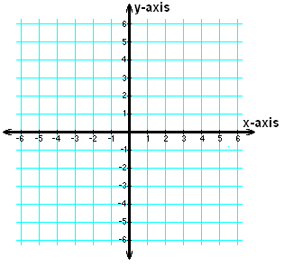
For the plane, an infinite two-dimensional manifold, two distance coordinates, taken in perpendicular directions, uniquely define a point (see below). The system, usually using x and y for the directions of coordinates, or axes, is called the Cartesian system. Points are found by following the x-axis for a distance b, and then moving perpendicularly (parallel to the y-axis) some distance c. The point is labeled (b,c).
For the aforementioned disc, the angular and linear (distance) systems are combined.

The figure above is essentially equivalent to the circular system mentioned previously, with one exception. An additional coordinate, r, is added to denote the distance from the center O of the disc. In reality, the distance r can be arbitrarily large, and the disc therefore infinite, making the angular-linear or polar coordinate system work for the plane as well. However, the restriction of r to being less than or equal to the radius of the disc emphasizes the different construction of the polar system versus the Cartesian system, and how it builds off the circular coordinate system.

The final simple possibility is the double angular or spherical system, shown above. It expands off the angular system of the circle, constructing another plane perpendicular to the plane containing the circle. The angle of elevation off the plane serves as the second angle, θ, in addition to the original circular angle, φ.
For three dimensions, there are several more cases.

The first is the triple linear system, with three axes, x, y, and z. Distances in the direction of each axis are given to uniquely determine a point. (negative coordinates signify movement in the opposite direction)

The second possibility is a system with two linear coordinates and one angular coordinate. A manifold using this system is the solid cylinder, or rod. The rod system is based off the disc system, with the angular and first linear coordinates defining a disc, and the second linear coordinate defining distance up the rod. In the above views, the rod is not solid, and instead two circular cross sections are shown to emphasize the first linear dimension. If one was to disregard the first linear dimension, a normal cylinder would result, and this is therefore another possibility for the two dimensional angular system. Consequently, the cylinder is a 2-manifold, and the rod is a 3-manifold. Again, both linear dimensions are restricted to finite values for emphasis.

The system with two angular coordinates and one linear coordinate is the ball system, as the ball is the simplest manifold with this system. The ball, as previously mentioned, is simply a solid sphere, with identical angular dimensions. A (restricted) linear dimension is added to denote the distance from the center of the ball, uniquely identifying a point.
The final possibility is the notion of a system with three angular coordinates. Following the pattern of the circle and the sphere, this manifold should also be the set of points equidistant to a fixed point. The set of manifolds with this property are generally called n-spheres, where n is the number of dimensions in the manifold. The circle is then the 1-sphere, the sphere the 2-sphere, and this new manifold, the 3-sphere. However, the full geometry of the three-sphere cannot be expressed with three dimensions, and instead requires four to reveal its curvature.
This generation of manifolds can continue indefinitely through any dimension, but the above process only produces a limited number of manifolds, i.e. the simplest of every dimension. Also, there are multiple possibilities for each system, with the disc and cylinder being one example given above. There are many other similar pairs in higher dimensions when one changes the orientation of the linear and angular dimensions.
Coordinates are necessary in performing mathematical operations on manifolds, and in mapping between them. The differences between angular and linear coordinates, and the number of dimensions needed to express them open the gates to a limitless world of surfaces, which the above method has only begun to explore. For the next post, see here.
Sources: http://www.ibiblio.org/links/devmodules/shared/html/glossary.html, http://www.mathematic.ws/, http://en.wikipedia.org/wiki/Spherical_coordinate_system, Visual Complex Analysis by Tristan Needham,
Another way to define a unique point on a manifold is by the use of coordinate systems. Coordinate systems are collections of numbers (a1, a2... an) that tell one how to identify a point uniquely. There are a number of ways to do this, but within each and every system lies the dimension of the manifold, for the number of coordinates needed to define a point uniquely is the same as the number of dimensions of the manifold.
There are many possible coordinate systems, and some may be more effective on some manifolds than on others. Consider the circle, the simplest of all manifolds.

The circular coordinate system (click to enlarge). The angle "a" uniquely determines a point on the circle, and the circle is therefore a one-dimensional manifold. Note that, similar to the difference between the sphere and the ball, the circle is only the line itself, while the interior of the plane defined by the circle is known as a disc. a is taken to be an angle between 0 and 2π if each point on the circle is to have a unique coordinate.

A similar process works for the line, an infinite manifold where the (signed) distance from 0 defines a unique point. The above is also called the number line.
For two dimensions, one can combine distance and angle coordinates in several combinations.
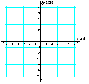
For the plane, an infinite two-dimensional manifold, two distance coordinates, taken in perpendicular directions, uniquely define a point (see below). The system, usually using x and y for the directions of coordinates, or axes, is called the Cartesian system. Points are found by following the x-axis for a distance b, and then moving perpendicularly (parallel to the y-axis) some distance c. The point is labeled (b,c).
For the aforementioned disc, the angular and linear (distance) systems are combined.

The figure above is essentially equivalent to the circular system mentioned previously, with one exception. An additional coordinate, r, is added to denote the distance from the center O of the disc. In reality, the distance r can be arbitrarily large, and the disc therefore infinite, making the angular-linear or polar coordinate system work for the plane as well. However, the restriction of r to being less than or equal to the radius of the disc emphasizes the different construction of the polar system versus the Cartesian system, and how it builds off the circular coordinate system.

The final simple possibility is the double angular or spherical system, shown above. It expands off the angular system of the circle, constructing another plane perpendicular to the plane containing the circle. The angle of elevation off the plane serves as the second angle, θ, in addition to the original circular angle, φ.
For three dimensions, there are several more cases.

The first is the triple linear system, with three axes, x, y, and z. Distances in the direction of each axis are given to uniquely determine a point. (negative coordinates signify movement in the opposite direction)

The second possibility is a system with two linear coordinates and one angular coordinate. A manifold using this system is the solid cylinder, or rod. The rod system is based off the disc system, with the angular and first linear coordinates defining a disc, and the second linear coordinate defining distance up the rod. In the above views, the rod is not solid, and instead two circular cross sections are shown to emphasize the first linear dimension. If one was to disregard the first linear dimension, a normal cylinder would result, and this is therefore another possibility for the two dimensional angular system. Consequently, the cylinder is a 2-manifold, and the rod is a 3-manifold. Again, both linear dimensions are restricted to finite values for emphasis.

The system with two angular coordinates and one linear coordinate is the ball system, as the ball is the simplest manifold with this system. The ball, as previously mentioned, is simply a solid sphere, with identical angular dimensions. A (restricted) linear dimension is added to denote the distance from the center of the ball, uniquely identifying a point.
The final possibility is the notion of a system with three angular coordinates. Following the pattern of the circle and the sphere, this manifold should also be the set of points equidistant to a fixed point. The set of manifolds with this property are generally called n-spheres, where n is the number of dimensions in the manifold. The circle is then the 1-sphere, the sphere the 2-sphere, and this new manifold, the 3-sphere. However, the full geometry of the three-sphere cannot be expressed with three dimensions, and instead requires four to reveal its curvature.
This generation of manifolds can continue indefinitely through any dimension, but the above process only produces a limited number of manifolds, i.e. the simplest of every dimension. Also, there are multiple possibilities for each system, with the disc and cylinder being one example given above. There are many other similar pairs in higher dimensions when one changes the orientation of the linear and angular dimensions.
Coordinates are necessary in performing mathematical operations on manifolds, and in mapping between them. The differences between angular and linear coordinates, and the number of dimensions needed to express them open the gates to a limitless world of surfaces, which the above method has only begun to explore. For the next post, see here.
Sources: http://www.ibiblio.org/links/devmodules/shared/html/glossary.html, http://www.mathematic.ws/, http://en.wikipedia.org/wiki/Spherical_coordinate_system, Visual Complex Analysis by Tristan Needham,
Monday, March 21, 2011
Manifolds: Mappings and Projection
To understand some terms used in this post, it is recommended that you first read Manifolds: Geometrically Equivalent vs. Topologically Equivalent.
The world of manifolds is extremely rich and diverse, especially when higher dimensions are considered. A multitude of objects can be explored, most of them fundamentally different from one another, and we are still very far away from identifying all of them, even in relatively low dimensions.
Note: Before exploring manifolds, it is useful to define "dimension" and what it means in terms of a manifold. Recall the definition of a manifold: any surface that appears "flat" at sufficiently small scale. However, "flat" is another word for Euclidean (or plane) geometry, and we can then define the dimension of a manifold as follows:
If a manifold resembles n-dimensional Euclidean space at sufficiently small scale, then it is an n-dimensional manifold.
As an example of this, consider a typical sphere, such as the Earth (the Earth is not exactly spherical, but is often used to represent the abstract mathematical sphere). To someone standing on the Earth, its surface appears to be a flat plane, i.e. two dimensional Euclidean geometry! Therefore, we conclude that the sphere is a two dimensional manifold, or 2-manifold.
Note: The term "sphere" only includes the surface of the sphere (or the Earth) and does not include the inside of the sphere. The region of three dimensional space bounded by the two dimensional sphere is known as the ball, and is a 3-manifold.
With the above clarification of terms, one notices that is easy to define the Earth as a 2-manifold. However, when one attempts to map the surface of the Earth on a flat surface, there are inevitable distortions.
As an example, consider the Mercator projection of the Earth.

When mapping the Earth onto a flat Euclidean plane, one must consider various geometrical properties of the sphere, including area, latitude and longitude lines, and lengths of these lines. A process called projection allows one to view a surface on a flat two dimensional plane. In the above case, a cylinder is used to project the Earth onto a plane (see image below).

For each point on the sphere, a line is drawn from the center of the sphere outward through the aforementioned point, and this line will eventually intersect with the cylinder (the cylinder does not actually have a "top" or a "bottom" but rather goes on forever). After all the points are mapped, the cylinder is unrolled into a plane, resulting in the fact that going off the right edge of the map goes to the left edge and vice versa. However, when one chooses a point near one of the poles, the line must go a large distance before intersecting the cylinder, and the poles themselves cannot be mapped at all! Despite these problems, this mapping is desirable for bearings, as it maps rhumb lines (or lines bearing in a specific direction, e.g. northwest, east southeast, etc.) and therefore also preserves angles.
Another (perhaps even simpler) useful projection for mapping the Earth (and especially mathematics) is the stereographic projection. It again maps the sphere onto a flat Euclidean plane, but in a different way. The figure below denotes this.

To project stereographically, a point of projection is first chosen. For the purposes of this example, the point of projection is always assumed to be the north pole. For each point on the sphere, a line is drawn from the north pole through this point, and is extended until it intersects the plane passing through the equator of the sphere. In mathematics, this is taken to be the complex plane (see here for a basic discussion of i and the complex plane) and the circle at which the sphere intersects the plane is taken to be the unit circle, i.e. the circle centered at 0 with radius 1.
The figure above shows two arbitrary points. Point A, on the plane outside the unit circle, corresponds to a point on the upper half of the sphere, while Point B, on the plane inside the unit circle, corresponds to a point on the lower half of the sphere. Points on the unit circle obviously remain in the same position. (1 and i are shown as examples)
Additional properties include the south pole of the sphere corresponds to the origin of the plane, and the north pole of the sphere does not correspond to ANY point on the normal plane. This is because the point of projection (the north pole) and the point to be projected (also the north pole) coincide, and the line is therefore a tangent line, which is parallel to the plane and never intersects it. The north pole is sometimes called infinity for this reason.

An image of the Earth using another type of stereographic projection where the plane of projection is tangent to the south pole of the sphere. In all other respects, this projection is similar to the one above; it still matches every point on the sphere with one point on the plane, with the exception of the north pole.
The stereographic projection has many properties that make it valuable to mathematics, the most important of which is that it preserves circles and angles (for a proof, see sources, specifically Needham). And since the points are projected continuously with a one-to-one correspondence, the mapping is a homeomorphism. Therefore, we can make the statement that
The Euclidean two dimensional plane is homeomorphic to the two dimensional sphere with one point removed.
The above reflects that the point of projection itself (the north pole in the above examples) cannot be projected onto the plane. In mathematics, it is possible to remedy this, by including infinity itself as a point on the complex plane, and the new entity that results is known as the extended complex plane. Infinity then corresponds to the north pole under stereographic projection. Note that the actual direction, in which we approach infinity does not matter, as all lines heading away from the origin will travel upwards on the sphere and eventually reach the north pole. In a sense, infinity is an endpoint of any straight line in the extended complex plane.
A generalized view on stereographic projection allows one to project from spheres of any dimension to their corresponding planes. For example, elliptic polychora, or four dimensional finite polytopes (see the polytopes series) are actually tilings of the three dimensional sphere which is the surface enclosing the four dimensional ball (this is the higher dimensional analog of the two dimensional sphere being a surface enclosing a three dimensional ball). Therefore, stereographic projection can be used in a similar way as the above to project such polychora onto flat Euclidean three space.

An example of a convex polychoron projected stereographically (specifically, it is the cantellated 24-cell, see here for more information)
Mappings and projection have revealed that the sphere and plane are fundamentally different, despite being members of the same dimension. Further posts in the manifolds series addresses this topic (see next post).
Sources: http://en.wikipedia.org/wiki/Stereographic_projection, Visual Complex Analysis by Tristan Needham, http://en.wikipedia.org/wiki/Mercator_projection
The world of manifolds is extremely rich and diverse, especially when higher dimensions are considered. A multitude of objects can be explored, most of them fundamentally different from one another, and we are still very far away from identifying all of them, even in relatively low dimensions.
Note: Before exploring manifolds, it is useful to define "dimension" and what it means in terms of a manifold. Recall the definition of a manifold: any surface that appears "flat" at sufficiently small scale. However, "flat" is another word for Euclidean (or plane) geometry, and we can then define the dimension of a manifold as follows:
If a manifold resembles n-dimensional Euclidean space at sufficiently small scale, then it is an n-dimensional manifold.
As an example of this, consider a typical sphere, such as the Earth (the Earth is not exactly spherical, but is often used to represent the abstract mathematical sphere). To someone standing on the Earth, its surface appears to be a flat plane, i.e. two dimensional Euclidean geometry! Therefore, we conclude that the sphere is a two dimensional manifold, or 2-manifold.
Note: The term "sphere" only includes the surface of the sphere (or the Earth) and does not include the inside of the sphere. The region of three dimensional space bounded by the two dimensional sphere is known as the ball, and is a 3-manifold.
With the above clarification of terms, one notices that is easy to define the Earth as a 2-manifold. However, when one attempts to map the surface of the Earth on a flat surface, there are inevitable distortions.
As an example, consider the Mercator projection of the Earth.

When mapping the Earth onto a flat Euclidean plane, one must consider various geometrical properties of the sphere, including area, latitude and longitude lines, and lengths of these lines. A process called projection allows one to view a surface on a flat two dimensional plane. In the above case, a cylinder is used to project the Earth onto a plane (see image below).

For each point on the sphere, a line is drawn from the center of the sphere outward through the aforementioned point, and this line will eventually intersect with the cylinder (the cylinder does not actually have a "top" or a "bottom" but rather goes on forever). After all the points are mapped, the cylinder is unrolled into a plane, resulting in the fact that going off the right edge of the map goes to the left edge and vice versa. However, when one chooses a point near one of the poles, the line must go a large distance before intersecting the cylinder, and the poles themselves cannot be mapped at all! Despite these problems, this mapping is desirable for bearings, as it maps rhumb lines (or lines bearing in a specific direction, e.g. northwest, east southeast, etc.) and therefore also preserves angles.
Another (perhaps even simpler) useful projection for mapping the Earth (and especially mathematics) is the stereographic projection. It again maps the sphere onto a flat Euclidean plane, but in a different way. The figure below denotes this.

To project stereographically, a point of projection is first chosen. For the purposes of this example, the point of projection is always assumed to be the north pole. For each point on the sphere, a line is drawn from the north pole through this point, and is extended until it intersects the plane passing through the equator of the sphere. In mathematics, this is taken to be the complex plane (see here for a basic discussion of i and the complex plane) and the circle at which the sphere intersects the plane is taken to be the unit circle, i.e. the circle centered at 0 with radius 1.
The figure above shows two arbitrary points. Point A, on the plane outside the unit circle, corresponds to a point on the upper half of the sphere, while Point B, on the plane inside the unit circle, corresponds to a point on the lower half of the sphere. Points on the unit circle obviously remain in the same position. (1 and i are shown as examples)
Additional properties include the south pole of the sphere corresponds to the origin of the plane, and the north pole of the sphere does not correspond to ANY point on the normal plane. This is because the point of projection (the north pole) and the point to be projected (also the north pole) coincide, and the line is therefore a tangent line, which is parallel to the plane and never intersects it. The north pole is sometimes called infinity for this reason.

An image of the Earth using another type of stereographic projection where the plane of projection is tangent to the south pole of the sphere. In all other respects, this projection is similar to the one above; it still matches every point on the sphere with one point on the plane, with the exception of the north pole.
The stereographic projection has many properties that make it valuable to mathematics, the most important of which is that it preserves circles and angles (for a proof, see sources, specifically Needham). And since the points are projected continuously with a one-to-one correspondence, the mapping is a homeomorphism. Therefore, we can make the statement that
The Euclidean two dimensional plane is homeomorphic to the two dimensional sphere with one point removed.
The above reflects that the point of projection itself (the north pole in the above examples) cannot be projected onto the plane. In mathematics, it is possible to remedy this, by including infinity itself as a point on the complex plane, and the new entity that results is known as the extended complex plane. Infinity then corresponds to the north pole under stereographic projection. Note that the actual direction, in which we approach infinity does not matter, as all lines heading away from the origin will travel upwards on the sphere and eventually reach the north pole. In a sense, infinity is an endpoint of any straight line in the extended complex plane.
A generalized view on stereographic projection allows one to project from spheres of any dimension to their corresponding planes. For example, elliptic polychora, or four dimensional finite polytopes (see the polytopes series) are actually tilings of the three dimensional sphere which is the surface enclosing the four dimensional ball (this is the higher dimensional analog of the two dimensional sphere being a surface enclosing a three dimensional ball). Therefore, stereographic projection can be used in a similar way as the above to project such polychora onto flat Euclidean three space.

An example of a convex polychoron projected stereographically (specifically, it is the cantellated 24-cell, see here for more information)
Mappings and projection have revealed that the sphere and plane are fundamentally different, despite being members of the same dimension. Further posts in the manifolds series addresses this topic (see next post).
Sources: http://en.wikipedia.org/wiki/Stereographic_projection, Visual Complex Analysis by Tristan Needham, http://en.wikipedia.org/wiki/Mercator_projection
Wednesday, March 9, 2011
Manifolds: Geometrically Equivalent vs. Topologically Equivalent
A manifold is the general term for a geometric figure, surface, or space. Manifolds can be of any dimension, and of are great importance in mapping, and in mathematics.
The study of the manipulation of surfaces is known as topology. It is very important to understand that geometry and topology, although both dealing with geometric figures, are very different. Geometry is concerned with sizes and shapes, i.e. measuring area, radius, perimeter, volume, and so forth. However, topology, which is more relevant to this post, does not worry about specific shapes. The following definitions are very important distinctions.
Geometrically equivalent: Two objects are geometrically equivalent if they have exactly the same size, shape and dimension. Figures with this property are called congruent. Another identical statement is that if two figures can be placed on top of each other to exactly line them up, then they are congruent.
Homotopic: Two objects are homotopic if they can be continuously deformed into one another. This means that the stretching, bending or twisting of an object does not alter it topologically. Two objects that can be continuous deformed into each other in this way are called homotopic to one another. Therefore, there exists what is called an invariant in the original surface. An invariant is defined in this sense as a feature of a manifold that remains the same when it is changed is some way. The specific example of this for two homotopic manifolds is called a homotopy group.
There are actually several different homotopy groups, each of which defines features of a manifold. The simplest of these is called the fundamental group, which determines the number of holes in a surface. The mug and the torus below both have one hole in their surface; they are homotopic and equivalent topologically.


Another way to express the same idea is to consider a point on a manifold, and, starting from that point, trace any path on the given manifold, with one condition: the endpoint and the starting point of the path must coincide. When this happens, the path is called a loop. If all possible loops can be contracted into a point without leaving the given surface, than the surface has no holes and is what is called simply connected.

A demonstration that the sphere is simply connected. The loop shown, along with any other loop beginning from any other point on the sphere, can be contracted without leaving the surface.
Other surfaces, such as the torus, do not share this property.

An image of a regular torus, with three example loops drawn on its surface. It can easily be seen that some loops, such as c can be contracted to a point without leaving the surface. Others, such as a and b, cannot. Additional analysis of the set of loops on a surface yields the number of holes, known as the genus of a surface.

The triple torus is a manifold with genus 3.
The remaining homotopy groups are, simply put, higher dimensional generalizations of this. For example, the 2nd homotopy group deals with the cutting of spheres out of a surface, unlike the fundamental or first group, which deals with the cutting of circles. Therefore, there are infinitely many homotopy groups possible, each of which corresponding to a specific dimension. The "loops" for the 2nd homotopy groups will be surfaces, rather than lines, that can be contracted to a point. In addition, there is a equivalent for any dimension. For any specific manifold, the homotopy groups will assign an invariant (or a set of invariants if multiple groups are used) that identifies it as homotopic to any other manifold with an equivalent invariant.
Homeomorphic: However, the actual definition of topologically equivalent is even broader than this. Two manifolds are topologically equivalent if they are homeomorphic. Note that if two manifolds are homeomorphic, they are homotopic, but the reverse is not necessarily true.
Two manifolds are homeomorphic if there exists some function that maps each point on one manifold to a corresponding point on the other.

An example of a simple mapping (click the image to enlarge) of the number line x (red) to the number line y=x^2 (blue). Each point on x is mapped to a corresponding point on y (only the points x=1 and x=2, becoming y=1 and y=4, respectively, are shown). The above lines are actually manifolds related by the mapping y=x^2!
However, for two manifolds related by a mapping to be homeomorphic, the mapping must satisfy certain conditions, listed below. For the mapping function f that relates a set of points X to a corresponding set of points Y:
Some definitions are in order:
Continuous: Literally that each change in input causes only a small change in output. In other words, there cannot be any "jumps" or discontinuities in the function.
One-to-one: If the function f maps a point a in X to a specific point b in Y, then a is the only value in X that f maps to b.
Onto: Each value in Y corresponds to a point in X.
Inverse: The inverse of a function f is the mapping that undoes f. In other words, f maps X to Y, and the inverse of f maps Y to X.
Armed with the ideas of homotopic, homeomorphic, and mapping, one can begin to explore the world of manifolds. (see the next post)
Sources: http://en.wikipedia.org/wiki/Homotopy_groups and other various wikipedia titles, Visual Complex Analysis by Tristan Needham, The Poincare Conjecture by Donal O'Shea, http://www.regentsprep.org/Regents/math/algtrig/ATP5/OntoFunctions.htm, http://media.web.britannica.com/eb-media/58/96258-004-7747AF96.jpg
The study of the manipulation of surfaces is known as topology. It is very important to understand that geometry and topology, although both dealing with geometric figures, are very different. Geometry is concerned with sizes and shapes, i.e. measuring area, radius, perimeter, volume, and so forth. However, topology, which is more relevant to this post, does not worry about specific shapes. The following definitions are very important distinctions.
Geometrically equivalent: Two objects are geometrically equivalent if they have exactly the same size, shape and dimension. Figures with this property are called congruent. Another identical statement is that if two figures can be placed on top of each other to exactly line them up, then they are congruent.
Homotopic: Two objects are homotopic if they can be continuously deformed into one another. This means that the stretching, bending or twisting of an object does not alter it topologically. Two objects that can be continuous deformed into each other in this way are called homotopic to one another. Therefore, there exists what is called an invariant in the original surface. An invariant is defined in this sense as a feature of a manifold that remains the same when it is changed is some way. The specific example of this for two homotopic manifolds is called a homotopy group.
There are actually several different homotopy groups, each of which defines features of a manifold. The simplest of these is called the fundamental group, which determines the number of holes in a surface. The mug and the torus below both have one hole in their surface; they are homotopic and equivalent topologically.


Another way to express the same idea is to consider a point on a manifold, and, starting from that point, trace any path on the given manifold, with one condition: the endpoint and the starting point of the path must coincide. When this happens, the path is called a loop. If all possible loops can be contracted into a point without leaving the given surface, than the surface has no holes and is what is called simply connected.

A demonstration that the sphere is simply connected. The loop shown, along with any other loop beginning from any other point on the sphere, can be contracted without leaving the surface.
Other surfaces, such as the torus, do not share this property.

An image of a regular torus, with three example loops drawn on its surface. It can easily be seen that some loops, such as c can be contracted to a point without leaving the surface. Others, such as a and b, cannot. Additional analysis of the set of loops on a surface yields the number of holes, known as the genus of a surface.

The triple torus is a manifold with genus 3.
The remaining homotopy groups are, simply put, higher dimensional generalizations of this. For example, the 2nd homotopy group deals with the cutting of spheres out of a surface, unlike the fundamental or first group, which deals with the cutting of circles. Therefore, there are infinitely many homotopy groups possible, each of which corresponding to a specific dimension. The "loops" for the 2nd homotopy groups will be surfaces, rather than lines, that can be contracted to a point. In addition, there is a equivalent for any dimension. For any specific manifold, the homotopy groups will assign an invariant (or a set of invariants if multiple groups are used) that identifies it as homotopic to any other manifold with an equivalent invariant.
Homeomorphic: However, the actual definition of topologically equivalent is even broader than this. Two manifolds are topologically equivalent if they are homeomorphic. Note that if two manifolds are homeomorphic, they are homotopic, but the reverse is not necessarily true.
Two manifolds are homeomorphic if there exists some function that maps each point on one manifold to a corresponding point on the other.

An example of a simple mapping (click the image to enlarge) of the number line x (red) to the number line y=x^2 (blue). Each point on x is mapped to a corresponding point on y (only the points x=1 and x=2, becoming y=1 and y=4, respectively, are shown). The above lines are actually manifolds related by the mapping y=x^2!
However, for two manifolds related by a mapping to be homeomorphic, the mapping must satisfy certain conditions, listed below. For the mapping function f that relates a set of points X to a corresponding set of points Y:
- The function f must be continuous.
- The function f must be one-to-one.
- The function f must be onto.
- The inverse of f must be continuous.
Some definitions are in order:
Continuous: Literally that each change in input causes only a small change in output. In other words, there cannot be any "jumps" or discontinuities in the function.
One-to-one: If the function f maps a point a in X to a specific point b in Y, then a is the only value in X that f maps to b.
Onto: Each value in Y corresponds to a point in X.
Inverse: The inverse of a function f is the mapping that undoes f. In other words, f maps X to Y, and the inverse of f maps Y to X.
Armed with the ideas of homotopic, homeomorphic, and mapping, one can begin to explore the world of manifolds. (see the next post)
Sources: http://en.wikipedia.org/wiki/Homotopy_groups and other various wikipedia titles, Visual Complex Analysis by Tristan Needham, The Poincare Conjecture by Donal O'Shea, http://www.regentsprep.org/Regents/math/algtrig/ATP5/OntoFunctions.htm, http://media.web.britannica.com/eb-media/58/96258-004-7747AF96.jpg
Saturday, March 5, 2011
Gamma Rays
Gamma rays are the final type of radiation found on the electromagnetic spectrum. Gamma rays have the highest frequency and smallest wavelength of any radiation, and therefore also have the highest energy.
Gamma rays are powerful enough to penetrate most substances, and are powerful ionizers. The gamma ray spectrum involves wavelengths lower than one trillionth of a meter (less than .000000000001 meters).
This radiation is often produced as a byproduct of atomic decay, in which unstable atoms emit energy through gamma rays and other particles before settling to a stable state. Descriptions of some of these reactions can be found here.
Among the parts of the electromagnetic spectrum, gamma rays are comparatively rare. Few objects are powerful enough to give off high amounts of gamma ray energy. However, this radiation is very important on atomic scales, when atomic decay spontaneously converts mass into energetic photons, i.e. gamma rays. This is possible due to the well known mass-energy relation
E=mc^2
where E corresponds to energy, m to mass, and c a constant (the speed of light: 186282 miles per second). The meaning of this equation is that a certain amount of mass is equal to a certain amount of energy. During the early stages of the Universe, the temperature was sufficiently high that particles collided with their antiparticle counterparts. When they collide, they instantly annihilate each other, releasing energy. As energy, the reverse happened, with particles and antiparticles being spontaneously created. Now these reactions only take place in extreme conditions, such as on the edges of a black hole.
Despite this, astronomical gamma ray sources can still be found, and the closest is the Moon.

An image of the Moon taken by a gamma ray telescope. The gamma rays emitted from the Moon originate when other solar ionizing radiation, such as ultraviolet, hits the Moon and causes the excitation of heavy atoms, and this in turn, causes the emission of gamma rays. In contrast, the Sun is nearly invisible in the gamma ray spectrum, because it consists of very light atoms (mostly Hydrogen and Helium) that cannot be excited by ionizing radiation.
Other gamma ray sources include solar flares, the death of massive stars (through processes such as supernovae) and their remnants (neutron stars and black holes), as well as active galaxies. Galaxies are "active" if large amounts of infalling matter are feeding their central black hole, giving off enormous amounts of radiation. Most information on gamma ray bursts is theoretical, as little is actually known about their sources, and they usually are very distant.
Gamma ray bursts and their sources are some of the most fascinating areas of astronomy.
Sources: http://en.wikipedia.org/wiki/Gamma_ray, http://science.hq.nasa.gov/kids/imagers/ems/gamma.html, http://en.wikipedia.org/wiki/Timeline_of_the_Big_Bang, http://en.wikipedia.org/wiki/Mass–energy_equivalence
Gamma rays are powerful enough to penetrate most substances, and are powerful ionizers. The gamma ray spectrum involves wavelengths lower than one trillionth of a meter (less than .000000000001 meters).
This radiation is often produced as a byproduct of atomic decay, in which unstable atoms emit energy through gamma rays and other particles before settling to a stable state. Descriptions of some of these reactions can be found here.
Among the parts of the electromagnetic spectrum, gamma rays are comparatively rare. Few objects are powerful enough to give off high amounts of gamma ray energy. However, this radiation is very important on atomic scales, when atomic decay spontaneously converts mass into energetic photons, i.e. gamma rays. This is possible due to the well known mass-energy relation
E=mc^2
where E corresponds to energy, m to mass, and c a constant (the speed of light: 186282 miles per second). The meaning of this equation is that a certain amount of mass is equal to a certain amount of energy. During the early stages of the Universe, the temperature was sufficiently high that particles collided with their antiparticle counterparts. When they collide, they instantly annihilate each other, releasing energy. As energy, the reverse happened, with particles and antiparticles being spontaneously created. Now these reactions only take place in extreme conditions, such as on the edges of a black hole.
Despite this, astronomical gamma ray sources can still be found, and the closest is the Moon.

An image of the Moon taken by a gamma ray telescope. The gamma rays emitted from the Moon originate when other solar ionizing radiation, such as ultraviolet, hits the Moon and causes the excitation of heavy atoms, and this in turn, causes the emission of gamma rays. In contrast, the Sun is nearly invisible in the gamma ray spectrum, because it consists of very light atoms (mostly Hydrogen and Helium) that cannot be excited by ionizing radiation.
Other gamma ray sources include solar flares, the death of massive stars (through processes such as supernovae) and their remnants (neutron stars and black holes), as well as active galaxies. Galaxies are "active" if large amounts of infalling matter are feeding their central black hole, giving off enormous amounts of radiation. Most information on gamma ray bursts is theoretical, as little is actually known about their sources, and they usually are very distant.
Gamma ray bursts and their sources are some of the most fascinating areas of astronomy.
Sources: http://en.wikipedia.org/wiki/Gamma_ray, http://science.hq.nasa.gov/kids/imagers/ems/gamma.html, http://en.wikipedia.org/wiki/Timeline_of_the_Big_Bang, http://en.wikipedia.org/wiki/Mass–energy_equivalence
Subscribe to:
Posts (Atom)