Mars Science Laboratory

Mars Science Laboratory (MSL) is a NASA mission to Mars, whose goal is to search for organic material and microbial life on the Martian surface. To do this, the mission landed the rover Curiosity on Mars, whence it will navigate the surface and conduct scientific experiments.



The spacecraft successfully launched from Cape Canaveral, Florida on November 26, 2011. After leaving the Earth's atmosphere, it began a cruise stage that lasted until MSL approaches Mars in the summer of 2012. It successfully landed on the red planet on August 6, 2012.

This mission makes use of innovative technologies essential for any future landings on Mars. At over 2000 pounds, Curiosity is by far the largest Mars rover ever to be constructed, five times the size of the rovers Spirit and Opportunity of the early 2000's. In order to land intact on the Martian surface, a precision landing was necessary.

Previous rovers used inflatable airbags to cushion their landings, and simply bounced until settling to their destination. This did not allow high precision in landing. However, Curiosity is too large for such techniques, and made use of a more complicated landing sequence.



The landing procedure that was used to lower the Curiosity rover to the surface (click to enlarge). In the atmosphere, parachutes and braking thrusts were used to decelerate the craft. Then, a device known as a  sky crane lowered the rover to the ground on cables to ensure proper orientation.  Once Curiosity was safely on the surface, the crane detached and propelled itself away, as to not interfere with the rover.

After the landing, the first images sent back from Curiosity confirmed its position.



One of the first images from Curiosity showing the Martian surface. The venue from which the rover explored its environment was Gale Crater. This crater was selected due to the exposed sediment along its banks, which hold millions of years of Martian geologic history.

Over the next few days, the rover, remaining stationary, tested its scientific equipment, checking all of its instruments and cameras in preparation for its first motorized movement on the surface of Mars, which occurred on August 29.

On August 19, Curiosity performed its first sample analysis, using its on-board laser and spectral analyzer to determine its composition. In the following months, the rover conducted numerous experiments involving samples, both of soil and of atmosphere. In early November 2012, the atmosphere was found to contain an unusual concentration of heavy isotopes of its constituent elements (mainly carbon and oxygen, forming CO₂. This indicates that the lighter isotopes were lost to space in the distant past, and this could explain the thinness of the Martian atmosphere.

During the first few months of the mission, the rover also took weather data, identifying some meteorological events on Mars. Most changes were related to dust storms and whirlwinds, and in fact the dust was discovered to catalyze a convective process in the Martian atmosphere: the dust on the side of Mars facing the Sun is lifted by wind into the atmosphere where it warms it, causing a greater differential in temperature between one half of the Martian atmosphere and the other (where it is night). This causes a flow of air from the cool to the warm side, restarting the process.

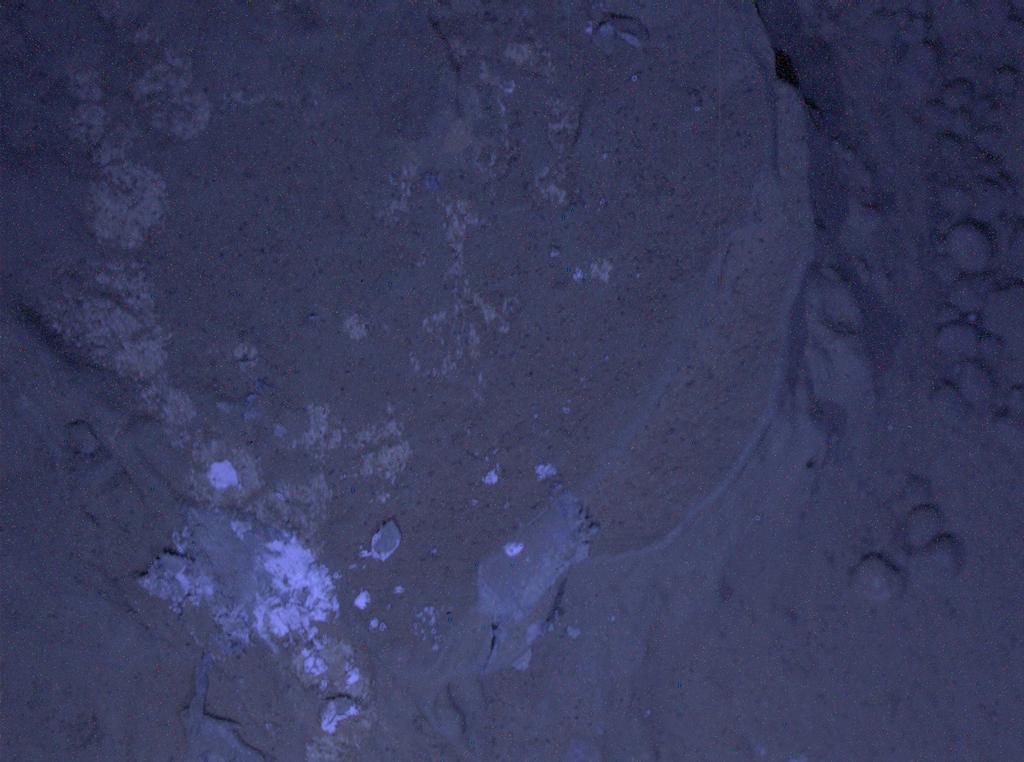
In January 2013, Curiosity imaged rocks at night, illuminating them with lights on the spacecraft. Using ultraviolet lamps, the rover searched for fluorescent minerals during the Martian night, at which time they would be visible (see image below).



In early February 2013, the rover completed its first drilling, obtaining a sample from several inches below the surface of bedrock. After obtaining a good number of rock samples and performing numerous other tests at Gale Crater, the rover prepared in June to begin a journey to its next destination, Mount Sharp. By the time Curiosity had spent one year on Mars in August 2013, it had already transmitted over 70,000 images, and had traveled about a mile along Mars's surface.

In October 2013, Curiosity performed a detailed analysis of the argon present in the Martian atmosphere, identifying the abundance of different isotopes. From this result, scientists deduced that some meteorites on Earth do indeed have their origin on Mars. Also, the prevalence (relative to on Earth) of a heavier isotope of argon suggests that Mars did undergo massive atmospheric loss earlier in its history. Early that December, scientists, using data collected by Curiosity announced that the rover had discovered evidence of an ancient lake (which last existed about 3.7 billion years ago) in Gale crater. Remarkably, this lake would have had very low salinity, and so, unlike most other similar findings, would have been nearly freshwater. This is significant as freshwater lakes could have supported a wider variety of life.

In March 2014, Curiosity began moving toward an interesting geological site known as "the Kimberley" (shown above). This gave the rover its first opportunity to conduct geological investigations of the several sandstone varieties (rather than mudstone, which it had been previously examining) to be found at the new site. It arrived at the site at the beginning of April and began analysis, including a new drilling in May.

On June 24, 2014, Curiosity completed scheduled its primary mission of one Martian year (687 Earth days). During this time, Curiosity systematically investigated the soil composition, radiation exposure, and abundance of organic molecules. At the time of the primary mission's completion, the evidence gathered by the rover was enough to confirm that the environment of Mars had once been favorable for "supporting microbial life".

Later in June, the rover moved out of its landing area into new terrain. It ultimately arrived at the base of Aeolis Mons (also called Mount Sharp), the mountain at the center of Gale Crater, in August. Exploration of the mountain is the primary goal for MSL's first mission extension. The 5.5 km (18,000 ft) high mountain was captured in the image below, taken by the rover:

Data gathered on the lower slopes of Mount Sharp in late 2014 included a series of sediment deposits which indicated the presence of a large lake at Gale Crater early in Mars's history that lasted tens of millions of years or more. This was the first major evidence for such a long-lasting, stable body of water on the red planet.

By early 2015, Curiosity had moved out of the bottom 33 feet of altitude of Mount Sharp and had entered a region with prominent mineral veins (as shown in the image above taken on March 18, 2015, which includes a scale). Such mineral veins forms when fluids move through cracks in existing rock and leave deposits. The light and dark minerals indicate a variety of fluid compositions.

In April 2015, the rover made another exciting discovery. Data from Curiosity indicated that water vapor condenses into liquid water in the Martian soil every night and reevaporates in the morning. Even though the Martian night temperatures are well below the normal freezing point of water (they may drop to -100°F), perchlorate salts in the soil reduce the freezing point of water (just as salting roads prevents them from freezing) enough that liquid water can form. This unexpected discovery suggests that a great deal more water could exist on Mars than previously thought.

The rover spent several months investigating sand dunes as it continued its journey, learning a great deal concerning the wind patterns on the planet's surface through the inspection of sand dune "ripples" (see below). The appearance of the sand dunes was comparable in appearance to those found on Earth.

After the sand dune investigation, Curiosity crossed the Naukluft Plateau towards the upward slopes of the mountain. This journey encompassed much of the first half of 2016, during which time the rover analyzed a few additional rock samples. During its investigation of Mount Sharp, Curiosity aimed to determine what geological environments are most suitable for the preservation of organic compounds and to identify geological layers and transitions. As well as being informative in their own right, these new objectives will guide future Mars missions.

On October 1, 2016, a second extension of two years to the mission began, allowing the rover to travel further up Mount Sharp. Later that month, Curiosity made an interesting discovery: a golf-ball sized meteorite on the Martian surface.

Laser spectrometry of this darkly colored rock indicated that it was primarily composed of iron, along with some nickel and phosphorus. This type of meteorite is usually formed from the core of asteroids. Further, the study of Mars meteorites allows the comparison between its population of impacting bodies and Earth's, revealing a great deal about how the inner Solar System evolved over time.

Early in 2017, an analysis of Curiosity data brought a curious paradox into focus by not making a particular expected discovery. While investigating what is believed to be an ancient lake floor, the rover did not discover significant carbonate minerals. It was expected that in Mars's early days, an atmosphere with more carbon dioxide allowed the trapping of heat by the greenhouse effect to melt ice into liquid lakes. Were this the case, some of the CO₂ would have dissolved in water, resulting in carbonates. However, no such discovery was made. This led scientists to seek alternate mechanisms for the presence of liquid water on early Mars.

In June 2017, a comprehensive study of Curiosity's findings at Gale Crater were assembled into a more complete picture of the ancient lake that existed there billions of years ago.

Of particular interest is the stratification of this lake, suggested by the differing mineral compositions of the "shallow" and "deep" walls of the crater. The stratification of lakes in this way is a phenomenon seen on Earth, and may have been conducive to different types of microbial life.

The next month, the rover began its investigation of Vera Rubin ridge, a geologic layer of Mount Sharp particularly rich in the iron oxide mineral hematite. The above image shows the location of this ridge as well as the rover's July 2017 position. Since hematite can form under wet conditions, analyzing the ridge revealed clues to Mars's ancient environments. Drilling at this site was difficult for Curiosity because an important part of the drill used to stabilize it as it pulverized rock stopped functioning back in December 2016. On the ridge, engineers experimented with a new drilling technique that did not require the stabilizers. This yielded results by early 2018, when the rover was able to obtain new samples.

In March 2019, Curiosity had the opportunity to capture Mars's small moons, Phobos and Deimos, as they passed in front of the Sun. This event is analogous to a solar eclipse on Earth, but the small size of Phobos and Deimos means that they cannot entirely block the Sun's disk. Therefore, they are known as transit events. The above animation shows a series of photographs of the Phobos transit. The photos are fascinating in their own right, but also help to refine our knowledge of the moons' orbits.

For years, the rover had made regular measurements of the concentrations of different gases in the Martian atmosphere in Gale Crater. As was known from previous missions, Mars's atmosphere is primarily (95%) CO₂, with trace amounts of nitrogen, argon, and oxygen gas. By analyzing variations over several revolutions around the Sun, it uncovered a seasonal pattern: the amount of nitrogen and argon fluctuated throughout the Martian year. These variations matched scientists' predictions, as they occurred in response to large amounts of carbon dioxide being frozen and unfrozen in the polar ice caps each year. However, the concentration of oxygen defied this pattern.

The above chart shows the expected seasonal variation in oxygen concentration as well as the observations of Curiosity at Gale Crater. It reveals an unexpected rise in oxygen during late spring and early summer, and an equally unexpected decline in winter. This behavior suggests a chemical process involving Martian soil, but it is so far unexplained.

In the summer of 2020, Curiosity left the "clay-bearing unit," the sedimentary layer it had been exploring for more than a year, and began to ascend even further to the "sulfate-bearing unit" above. Characterized by sulfate minerals such as gypsum, the rocks in this layer were likely formed through evaporation. To reach this new layer, however, the rover had to navigate around a mile-wide patch of sand. The composite image above (made from 116 individual photos) helped it to chart a course.

Sources: Mars Science Laboratory, Wikipedia, http://marsprogram.jpl.nasa.gov/msl/, http://mars.jpl.nasa.gov/msl/, http://www.npr.org/blogs/thetwo-way/2013/12/09/249760330/curiosity-finds-evidence-of-ancient-fresh-water-lake-on-mars?utm_content=socialflow&utm_campaign=nprfacebook&utm_source=npr&utm_medium=facebook, http://upload.wikimedia.org/wikipedia/commons/6/65/673885main_PIA15986-full_full.jpg, http://mars.nasa.gov/files/msl/2014-MSL-extended-mission-plan.pdf, http://www.nasa.gov/press/2014/december/nasa-s-curiosity-rover-finds-clues-to-how-water-helped-shape-martian-landscape/#.VItLjov4tFL, http://www.vox.com/2015/4/13/8384337/mars-water-liquid-curiosity, http://mars.nasa.gov/msl/news/whatsnew/index.cfm?FuseAction=ShowNews&NewsID=1912, http://mars.nasa.gov/news/2016/mars-rock-ingredient-stew-seen-as-plus-for-habitability&s=2, https://mars.nasa.gov/news/2017/nasas-curiosity-rover-sharpens-paradox-of-ancient-mars&s=2, https://mars.nasa.gov/news/curiosity-peels-back-layers-on-ancient-martian-lake/, https://mars.nasa.gov/news/curiosity-mars-rover-begins-study-of-ridge-destination/, https://mars.nasa.gov/news/8425/curiosity-captured-two-solar-eclipses-on-mars/, https://mars.nasa.gov/news/8704/curiosity-mars-rovers-summer-road-trip-has-begun/?site=msl

Infinity: The Aleph Sequence

This is the thirteenth and final post of the Infinity Series. For the first, see here. For all posts, see the Infinity Series Portal.

In the previous seven posts, the world of countable ordinals has been explored in depth, allowing one to taste its incomprehensible vastness. It is truly remarkable how merely taking 2 to the power of ℵ₀ could produce a uncountable cardinal so "easily", but that no number of additions, multiplications, exponentiations, or functions on ω could yield an uncountable ordinal. It is through such an examination that one begins to appreciate how inconceivably numerous are the real numbers and the members of the continuum in comparison to the rational and even algebraic numbers. Yet it is possible to go still further.

The first uncountable ordinal is the set of all countable ordinals, which, not being a member of this set, confirms that it is not countable. It is denoted ω₁ (note the similarity in notation to ω₁^CK, the Church-Kleene ordinal defined previously). The cardinality of ω₁ is denoted ℵ₁, the second ℵ number. Additionally, ω₁ is what is called the initial ordinal of the cardinal number ℵ₁, as it is the smallest ordinal with this cardinality (analogously, the initial ordinal of ℵ₀ is ω).

Before going on, it is useful to describe another property that ordinals and cardinals may possess. Every ordinal (or cardinal) can be regular or singular. To determine whether any quantity is regular or singular, one must consider the set which has the given quantity as its supremum. For example, consider the ordinal ω². It is equal to

sup{ω,ω*2,ω*3,...,ω*n,...},

and the set in question, namely {ω,ω*2,ω*3,...,ω*n,...}, has order type ω (recall that ordinals themselves each represent an order type, and each order type represents a special class of sets that can be reached from one another with a one-to-one order preserving correspondence). Since the order type of this set, ω, is not equal to the original ordinal, ω², ω² is singular. Note that, though, the set above has the same cardinality as ω², it does not have the same order type. In contrast, ω is a regular ordinal. All the sets which have it as a supremum are infinite sets of natural numbers, and it is easily to see that they all have order type ω.

For cardinals, the definition is even simpler. One simply considers the sets of cardinals that have the cardinal as a supremum, and evaluate the cardinality of the sets. If these sets have the same cardinality of the number, it is regular. Otherwise, it is singular. For example, ℵ₀ is the first infinite cardinal, and is the supremum of any infinite sequence of finite cardinal numbers, each of which have a cardinality of ℵ₀. This cardinal is therefore regular. The order type or cardinality of the set of which the given quantity is a supremum is the quantity's cofinality. For a successor ordinal or cardinal, the cofinality is defined as 1, e.g. the ordinal 5 is the supremum of the set {4}, which has order type 1.

The first few regular ordinals are 0 (trivially), 1, ω, and ω₁. ω₁ can be seen as regular by the following argument. We know that countable sequences of countable ordinals have only countable ordinals as suprema. Therefore, the order type of a set {α,β,γ,...}, whose supremum is ω₁, is an uncountable ordinal. However, if this ordinal were greater than ω₁, some element of the set would also have to be greater than ω₁. Therefore, the cofinality of ω₁ is itself, and the first uncountable ordinal is regular. The cardinals corresponding to these four ordinals are also regular.

Recall the previous definition of the cardinal beth-one, which was that this cardinal was the cardinality of the real numbers, and that it was the cardinality of the power set of the set of all natural numbers, i.e. 2^ℵ₀. It has been proven that the statement "beth-one is equal to aleph-one" is independent of ZF theory. The proposition that this statement is true is known as the continuum hypothesis. In other words, the continuum hypothesis states that

2^ℵ₀ = ℵ₁

This seems reasonable, given that both cardinals in the above equality were encountered in the context of being the "first" uncountable cardinal. For the purposes of this post, the two will be assumed to be equal simply in order to avoid dealing with the beth-sequence separately. Also, the generalized continuum hypothesis, that each subsequent member of the beth-sequence is equal to its corresponding aleph cardinal, will be assumed for clarity. However, the focus on the development of cardinals will be based on that of ordinals, and little is lost by assuming that the aleph- and beth-sequences are synonymous.

The next cardinal number after ℵ₁ (assuming the continuum hypothesis), is ℵ₂, which has an initial ordinal ω₂, both of which are by definition regular for the same reasons as ω₁. Similarly, all ordinals between ω₁ and ω₂, of which there are uncountably many, are singular.

Similarly, one can define a series of regular cardinals ℵ₀, ℵ₁, ℵ₂, ℵ₃, and in general ℵ_n for natural n, and a analogous sequence of ordinals ω, ω₁, ω₂, ω₃,...,ω_n.

The cardinal sup{ℵ₀,ℵ₁,ℵ₂,...,ℵ_n,...} is denoted ℵ_ω. The initial ordinal of this cardinal is ω_ω. Since the cofinality ω_ω is ω (there is one member in {ω,ω₁,ω₂,...,ω_n,...} has one member for each natural n), this ordinal, and ℵ_ω, are singular.

ℵ_ω is also the first so-called inaccessible cardinal, meaning that its ordinal subscript is a limit ordinal. Similarly, larger cardinals, such as ℵ_ω*2, and ℵ_ω², having limit ordinals as indices, are inaccessible. Next, we "number" these inaccessible cardinals with ordinals. For example, ℵ_ω is identified with 1, ℵ_ω*2 with 2, and so on. Therefore, ℵ_ω² is labeled as the ω-th inaccessible cardinal. Similarly, every cardinal ℵ_ω*α is labeled α, as every limit ordinal is a multiple of ω.

A cardinal is considered 1-inaccessible if its initial ordinal is the same as its label on the list of inaccessible cardinals. This means that if the cardinal is of the form ℵ_ω*α, its initial ordinal must be α. The first cardinal for which this holds is the supremum of the set

{ℵ_ω,ℵ_ωω,ℵ_ωωω,...},
whose initial ordinal is ω_ωω....
Clearly, removing an "ω" from this infinite chain does not change the value, nor does multiplying by ω on the left. Therefore, this cardinal is 1-inaccessible. The first 1-inaccessible cardinal is the limit of the ℵ notation in a sense, as it requires an infinite number of "ω's" to write. Similarly, other 1-inaccessible cardinals exist, and can be numbered with ordinals in the same fashion. A cardinal whose initial ordinal is the same as its label on the list of 1-inaccessible cardinals is called 2-inaccessible. And so larger and larger cardinals are defined that are 3-inaccessible, 4-inaccessible. Clearly, for α-inaccessible cardinal κ, κ is also β-inaccessible for all β < α. Therefore, one can define a cardinal as ω-inaccessible if it is 1-, 2-, 3-,... inaccessible for all natural numbers.

Then, the notion of α-inaccessibility can be defined for any α, with the limit ordinal case being treated similarly to ω-for a limit ordinal α, a cardinal is α-inaccessible if it is also β-inaccessible for all β < α.

Next, a cardinal is hyper-inaccessible if it has an initial ordinal α, and is α-inaccessible. Such a cardinal is immensely large, as, for all cardinals yet considered, their initial ordinals were far higher than their degree of inaccessibility. For example, for the 1-accessible cardinal above, the degree of inaccessibility is only 1, while the initial ordinal α is so large that ω_α = α. By substituting "hyper-inaccessible" for "inaccessible" in the definition of 1-inaccessible cardinals, i.e. by numbering the hyper-inaccessible cardinals, one obtains corresponding definitions for 1-hyper-inaccessible, 2-hyper-inaccessible, and, in general α-hyper-inaccessible cardinals. Finally, there are hyper-hyper-inaccessible cardinals, the process can repeat, generating hyper-hyper-hyper-inaccessible cardinals, and so on.

A Mahlo cardinal is then defined as a cardinal that is inaccessible, hyper-inaccessible, and so on for any finite number of "hyper-'s". This is an example of a cardinal that cannot be proved to exist without the use of a large cardinal axiom. Without such an axiom, it is impossible to prove that any cardinal satisfies the needed property to be considered Mahlo.

As one explores higher cardinals, and their corresponding ordinals, each type of cardinal tends to become associated with the axiom with which its existence can be proved. To confirm that larger cardinals exist, one generally needs stronger and stronger axioms. However, if an axiom becomes too strong, it can sometimes create an inconsistent system (paired with other axioms), where a statement and its negative can both be proved true. If such an axiom was confirmed to prove an inconsistency, it seems reasonable that it would be discarded, and with it, its corresponding cardinals.

Therefore, in a way, there does exist an "upper limit" for cardinals and ordinals based on the strength of their accompanying axioms. Note that this does not mean there is a highest ordinal or cardinal, because this is impossible (e.g., for any ordinal α, its successor α' is greater than α and is also an ordinal). The situation is analogous to that of countable ordinals: there is no highest countable ordinal, yet the set of countable ordinals does have an upper limit, ω₁. In the case of the totality of cardinals and ordinals, there is probably even more "room to maneuver" below the upper limit, and plenty of cardinals not yet discovered.

The task of determining the hierarchy of large cardinals is ongoing and will not be discussed in detail here. However, the above description gives an idea of how such cardinals are defined. In conclusion, the realm of infinities, despite the insight provided by the use of cardinals and ordinals, is still not completely explored, and increasingly ingenious methods will be required to generate higher and higher quantities. The possibilities-as one would expect-are infinite!

Sources: Regular Cardinal, List of Cardinal Properties, etc., Wikipedia

---

Author's Note (March 29, 2012): Of all my endeavors concerning this blog to date, the Infinity Series was perhaps the most ambitious, and definitely the most difficult. To attempt to convey even a glimpse of infinite sets and set theory is a challenging task. The above is far from an authoritative reference, and much is omitted where explanation would require the addition of large amounts of new material. Moreover, the mathematical arguments are less than rigorous, and the so-called "proofs" are often but sketches of their full versions-which require whole sets of axioms to complete.

Nevertheless, I am hopeful that this nuanced approach to a very narrow area of mathematics allows at least limited accessibility to those not acquainted with the nuts and bolts of set theory. For all my visitors, thank you for reading.

Professor Quibb

Infinity: Beyond Recursive Ordinals

This is the twelfth and penultimate post of the Infinity Series. For all posts, see the Infinity Series Portal.

In the previous post, the idea of an ordinal collapsing function was expanded to produce a series of these functions, each corresponding to a natural number. One could go even further listing fixed points and identifying ordinals inaccessible from certain operations and functions, but this is tedious, and is of little interest. To identify further ordinals beyond those accessible with a method involving fixed points, one must use a totally new idea.

Though set theory was mentioned as the basis for all subject matter in this series, no rigorous definition was ever made of any part of this theory. Rather, it has been assumed that the sets mentioned can be defined and constructed. However, set theory is based on assuming a few intuitively obvious or underlying statements that are accepted as being true. These are known as axioms. Formulae derived from these axioms or combinations thereof are then true statements.

However, there is no one "correct" set of axioms from which to assemble a theory that simultaneously has two desirable qualities: consistency and completeness. A consistent theory contains no two statements contradicting one another, i.e. if, for some statement p, "p is true" is derivable from the axioms "p is false" is not. In contrast, a complete theory is such that every statement p can be proved either true or false from the axioms. It was proved by Gödel in his incompleteness theorems that a set theory incorporating arithmetic cannot be simultaneously consistent and complete.

Therefore, there is a multiplicity of possibilities for the selected axioms, with no one clearly the "best", and, correspondingly, there are many different varieties of set theory. Of interest here are the axioms involved in the construction of sets. One basic axiom present in many variations of set theory is the pairing axiom, which, in logical notation, is

∀A∀B∃C∀D(D ∈ C↔(D = A∨D = B)).

In this axiom, A, B, C, and D are set variables, meaning that they take as values sets only, ∀ is the universal quantifier, read "for all", ∃ is the existential qualifier, meaning "there exists", ∈ is the membership relation, ↔ is the biconditional meaning "if and only if", and ∨ is the logic gate "or". Therefore, in common english, the axiom of pairing states:

"For all sets A and B, there exists a set C such that for all sets D, D is a member of C if and only if D is equal to A or D is equal to B."

This can be further paraphrased to "For any two sets, there is a third containing only the two as members", which simply allows one to create a set with a given two members, hence the name "pairing". Together with the definition {S,S} = {S}, which simply means that redundant elements in a set are deleted, one can construct the ordinals 1 and 2 from 0 through the axiom of pairing. 1 = {0} is derived from the case A = B = 0 in the axiom, as C is then {0} = 1. Furthermore, if A = 0 and B = 1, then the axiom guarantees the existence of the set {0,1} = 2. However, the ordinal 3 cannot be constructed in the same fashion, as it has more than two members. Therefore, the axiom of union, another axiom useful in constructing sets, is introduced:

∀A∃B∀C(C ∈ B↔∃D(C ∈ D∧D ∈ A))

This axiom collects all sets C such that C is a member of a member of A into a set B, known as the union of A. Note the relation to the definition of union we have already seen: the operation of union, when applied to multiple sets, collects their members; similarly, the union of a single set is the union of all its members. For example, the union of the set {{Ø},{{Ø}},{Ø,{Ø}} = {{0},{1},{2}}, the members of which are all guaranteed to exist by the axiom of pairing is the same as the union of its members, namely {0}∪{1}∪{2} = {0,1,2} = 3. By use of these two axioms, any finite ordinal can be constructed.

There is a third important axiom, called the axiom of infinity, which grants the existence of an infinite set, specifically the ordinal ω. Without it, one can not prove that infinite ordinals exist, and ω, the first ordinal that cannot be proven to exist, is called the strength of the theory. Strictly speaking, even some theories without the axiom of infinity "know" that ω exists, i.e. know that there is a set of natural numbers, but cannot prove that it is well-ordered, and thus cannot confirm its status as an ordinal. Thus far, the axioms discussed have been part of the theory known as Zermelo-Frankel Set Theory, or ZF set theory. The strength of this theory is measured by an ordinal higher than any ordinal so far discussed, as ZF set theory includes the concepts of function, fixed point, and (to a limited extent) inaccessibility. Therefore, all the processes used to describe ordinals thus far are "embedded" in ZF, and all the ordinals stated thus far can be explicitly constructed.

Technically, this new ordinal, which we shall call the ZF-ordinal, is not an ordinal at all, at least in ZF theory, where we cannot even confirm its status as an ordinal. This is an example of incompleteness in ZF theory. In order to prove that the ZF-ordinal, which contains all countable ordinals constructed thus far, is an ordinal, one must add additional axioms to ZF to strengthen the theory, and augment its ability to construct ordinals. But what axioms should be added? The type of axioms that serve this purpose are called large cardinal axioms, and confirm the existence of cardinals with certain properties. It seems somewhat odd that axioms concerning cardinal numbers would have anything to do with constructing ordinals. However, of the most importance are the properties themselves of the cardinals, which outline new methods for constructing ordinals.

The precise forms of these axioms will not yet be explained, as they do pertain to large cardinals that have not yet been discussed, but we will outline the hierarchy which they form. The first large cardinal axiom will be called A1, and is independent of ZF set theory, i.e. cannot be proved true or false by the existing axioms. Therefore, a new theory consisting of the original axioms and A1 is formed, which will be denoted ZFA1. This new theory can construct the ZF-ordinal, and even higher countable ordinals at that. The set of ordinals that can be constructed in this theory is again an ordinal, and by definition, its status as an ordinal is indeterminate within ZFA1. It is called the ZFA1-ordinal. By assuming more axioms A2, A3,..., one can obtain higher ordinals, and correspondingly "higher" set theories ZFA2, ZFA3,..., each of which has a higher corresponding strength. The ordinals defined in this way are called (rather paradoxically) unrecursible recursive ordinals, referring to the fact that they cannot be defined by recursive functions within the given theory, but rather require the theory itself in their definition.

From here one can set up a hierarchy of axioms. For any two axioms of this type, X and Y, either the two are "equal" in that they can be proved to imply one another, or one is stronger than the other, and augments ZF to yet a stronger set theory. The limit of the strength of the successive theories in this way may be further increased by using so-called axiom schemata (singular schema), which introduce additional variables into the logical statement. An axiom schema asserts that the given statement is true for all values of the variable. Also, meta-axioms, namely procedures for finding more axioms can extend the hierarchy even further. Eventually, a point is reached where no strengthened version of ZF or any other type of function can generate an ordinal. This inaccessible limit is called the Church-Kleene ordinal, and is written ω₁^CK.

ω₁^CK is the set of all recursive ordinals, and is then an ordinal, although it cannot be proven that this is true in any of the theories yet described. One could say that this ordinal's definition is based on those smaller than it and is therefore recursive, but this is not true, as the system of recursion itself is within the definition. Additionally, ω₁^CK could have served as the Ω in the previously discussed ordinal collapsing functions (see here), though, technically speaking, the ZF-ordinal or any others of the "unrecursible recursive" variety would have served as well. ω₁^CK is often chosen simply because its definition is simpler and more elegant.

Remarkably, ω₁^CK is still countable. This can be seen by considering the fact that there are only countably many notations through which to define ordinals; for each function considered thus far, each can take only countably many arguments, and there are only countably many functions based off of countable ordinals. Since all recursive notations are exhausted on countable ordinals, ω₁^CK is countable. Nor is it the last countable ordinal. One can of course create the set including all recursive ordinals and ω₁^CK, which is the ordinal ω₁^CK + 1, and so on.

In fact, one can define the set of all ordinals accessible from functions on all ordinals including the Church-Kleene ordinal, which is some other limit ordinal that could have served as Ω₂. Furthermore, by repeatedly define inaccessible ordinals, one can obtain a sequence of countable ordinals, each of which is greater than any recursive function on the previous one, and is parallel to the Ω sequence.

There is no end to this process, and one can generate as many countable ordinals as desired in a similar fashion. However, no matter how far one goes with defining countable ordinals, one can only reach an infinitesimal fraction of them, as functions defined within the countable ordinals always produce still more countable ordinals. The situation is analogous to that of whole numbers: one can always define a larger one, but there are always still infinitely more. How, then, can one work with uncountable ordinals and their cardinal counterparts? These problems will be addressed in the next post.

Sources; http://projecteuclid.org/DPubS/Repository/1.0/Disseminate?handle=euclid.pl/1235418473&view=body&content-type=pdf_1,
Axiomatic Set Theory by Patrick Suppes, A New Kind of Science by Stephen Wolfram

Infinity: Extended Collapsing Functions

This is the eleventh post of the Infinity Series. For the first, see here. For all posts, see the Infinity Series Portal.

In the previous post, an ordinal collapsing function was used to access high ordinals. However, all the outputs of the function discussed so far are alternatively expressible as Veblen functions with finite numbers of arguments. It was also seen that ψ(Ω^Ωα) is equal to the supremum of all ordinals that can be represented by an α + 1-argument Veblen function. This continues up to
ψ(Ω^Ωω), the first ordinal requiring infinite arguments to represent in Veblen notation. Being the supremum of countably many countable ordinals, it is countable, and is known as the small Veblen ordinal, though this ordinal is of course nothing near small.

In fact, it is small only when compared to even larger ordinals, such as the large Veblen ordinal, which is equal to ψ(Ω^ΩΩ). Alternatively, this ordinal represents the supremum of all others writable in Veblen notation of infinitely many, but only predicatively many, arguments. In short, since Veblen functions of high numbers of arguments are built off of those with lower numbers of arguments, only predicative ordinals, or those can be defined using lower ordinals alone, can serve as the number of arguments for such a function. Since Ω is clearly larger than any predicative ordinal, ψ(Ω^ΩΩ) is the supremum of the entire system of Veblen notation.

However, the ordinal collapsing function goes still further, defining ψ(Ω^ΩΩΩ), and in general ψ(Ω↑↑n) for finite n. Eventually one reaches the value ψ(ε_{Ω + 1}). The function is finally permanently stuck here, as ε_{Ω + 1} is not constructible from the original set S, and cannot be generated to plug to the ψ function. It is therefore never a member of the set C(α) no matter the value of α. ψ(ε_{Ω + 1}) is known as the Bachmann-Howard ordinal.

To go further using ordinal collapsing functions, we define a second function ψ₁, the value of ψ₁(α) being the smallest ordinal that cannot be finitely constructed using addition, multiplication, exponentiation, the original ψ function and ψ₁|_α, or the ψ₁ function restricted to α, these operations beginning from the set T₁ = {0,1,...,ω,...,Ω,Ω₂}, where Ω₂ is an ordinal higher than any of those that will be constructed with the ψ₁ function, and consequently, higher than Ω (again, it is not necessary for the definitions of Ω and Ω₂ to be in any way precise). Also, T₁ is assumed to contain all ordinals up to and including Ω, although we have no way yet of characterizing these ordinals, and so the definition is once again impredicative.

ψ₁(0) is clearly just ε_{Ω + 1}, as ψ₁|₀ is degenerate and has no values. But since all the ordinals less than Ω are in T₁, none of these can be equal to ψ₁(0), and since the ψ function only produces ordinals less than Ω, the first ordinal that is inaccessible is simply the limit of normal operations on Ω, namely ε_{Ω + 1}. Note that this is not the Bachmann-Howard ordinal, but a much larger indefinite quantity, the Bachmann-Howard ordinal being the ψ function at this value,
ψ(ε_{Ω + 1}). In fact, we cannot even be assured of the countability of ε_{Ω + 1}, due to the vagueness with which Ω was defined. Next,

ψ₁(1) = ε_{Ω + 2},

with the last term being the upper limit of iterated exponentiation on ε_{Ω + 1}. Now we return to the original collapsing function ψ, and modify its definition as follows:

ψ(α) is the first ordinal that cannot be constructed from the set S₁ = {0,1,ω,Ω,Ω₂} using the operations addition, multiplication, exponentiation, ψ|_α, and ψ₁.

Note no restriction is necessary on ψ₁ in this definition, as ψ₁ only produces values strictly greater than Ω, which is in turn greater than any ordinal produced by the ψ function. The outputs of ψ₁ therefore cannot affect which ordinal assumes the value of ψ(α), no matter its domain. This new definition produces values identical to those produced by the old for all ψ(α) such that α ≤ ε_{Ω + 1}, and using the same notation therefore produces no ambiguity. However, ψ(ε_{Ω + 1} + 1) is not equal to the Bachmann-Howard ordinal for this definition, since ε_{Ω + 1} is in C(ε_{Ω + 1} + 1). ψ(ε_{Ω + 1} + 1) is then equal to the next epsilon number after the Bachmann-Howard ordinal, namely

ε_{ψ(ψ1(0)) + 1} = ε_{ψ(εΩ + 1)) + 1}

One can go on through ψ(ψ₁(0) + 2), ψ(ψ₁(0) + Ω), and so on, on up to
ψ(ψ₁(1)) = ψ(ε_{Ω + 2}). Returning to ψ₁, ψ₁(2) = ε_{Ω + 3}, and in general
ψ₁(α) = ε_{Ω + 1 + α}, for all α up through Ω (with ψ₁(Ω) = ε_Ω*2) and beyond. Each of these can be plugged into the ψ function to yield yet another large countable ordinal, some of which are ψ(ψ₁(ψ₁(0))), ψ(ψ₁(ψ₁(ψ₁(0)))), and so on. Since each nested ψ₁ essentially iterates the ε function on Ω + 1, the limit of these expressions yields the first fixed point of such iteration, in other words the first α such that ψ₁(α) = α. This ordinal is ζ_{Ω + 1}, hence ψ₁(ζ_{Ω + 1}) = ζ_{Ω + 1}.

In a situation analogous to the original ψ function, ψ₁ is temporarily stuck at ζ_{Ω + 1}, as ζ_{Ω + 1} requires infinite steps to produce from T₁. ψ₁(α) is then fixed from ζ_{Ω + 1} on up to Ω₂, with ψ₁(Ω₂) still equal to ζ_{Ω + 1}, but ψ₁(Ω₂ + 1) is larger, as the domain of the restricted function ψ₁|_{Ω2 + 1} includes Ω₂, which is in T₁. ψ₁ is developed further in a similar way, a few notable values being

ψ₁(Ω₂*2) = ζ_{Ω + 2},
ψ₁(Ω₂²) = η_{Ω + 1}, and
ψ₁(ε_{Ω2 + 1}),

with the last being the highest value attainable by the ψ₁, as the function is constant afterward, in the same fashion as ψ is after ε_{Ω + 1}. Therefore,
ψ(ψ₁(ε_{Ω2 + 1})) is the highest ordinal accessible by the current definition of ψ, but is still much less than Ω.

Of course, there is no need to stop here. One can introduce a third function ψ₂, with ψ₂(α) the smallest ordinal not constructible from the set T₂ = {0,1,...,ω,...,Ω,...Ω₂,Ω₃}, in other words the set that contains all ordinals up to and including Ω₂, as well as an additional ordinal Ω₃, which is an arbitrary ordinal higher than any value that ψ₂ will attain.

ψ₂(0) is then equal to ψ(ψ₁(ε_{Ω2 + 1})). The definition of subsequent values of ψ₂ is as follows

ψ₂(α) is the smallest ordinal inaccessible from the operations of addition, multiplication, exponentiation, ψ, ψ₁, and ψ₂|_α from the set T₂.

One then alters the definitions of ψ₁, and finally, ψ, analogously in order to admit values such as ψ(ψ₁(ψ₂(Ω))), which is far greater than any ψ ordinal yet discussed, but of course considerably less than Ω. One can continue to generalize these functions, defining ψ₃, ψ₄, and so on, and each time altering all previous definitions accordingly. For natural numbers i and j, the function ψ_i adjusted for all ψ functions up to j, with j ≥ i, is written as ψ_ij. The general definition below is true for all functions ψ_ij (with the original ψ replaced by ψ₀ for clarity):

ψ_ij(α) is the smallest ordinal not constructible through a finite series of the operations addition, multiplication, exponentiation, ψ₀, ψ₁,..., ψ_i|_α, ψ_{i + 1},..., ψ_j on any elements of the set {0,1,...,ω,...,Ω,...Ω₂,...,Ω_i,Ω_{i + 1},...,Ω_j}, where each Ω_k is an arbitrary ordinal larger than any constructible with the function ψ_{k - 1}.

To understand this general definition, a few observations must be made. First, due to the definition of Ω_k, it is higher than any ordinal constructible with the previous ψ function. Therefore, the only restricted function in the definition is the one that is being defined, namely ψ_i, which produces ordinals strictly below Ω_i. Since the other ψ functions stay within their respective ranges also, they cannot (by themselves) produce a value in this range, and cannot directly affect ψ_i(α). Also, the purpose of the value j is simply to identify how "upgraded" each ψ function is, e.g., the difference between the initial definition of ψ (ψ₀) versus its "upgraded" definition incorporating ψ₁. Moreover, the set from which the ordinals are being constructed includes all ordinals up through Ω_i, but afterwards only the Ω ordinals between i and j.

Finally, the purpose of this multitude of functions is merely to plug them back in to ψ in order to generate further values, all of which are still far less than Ω. The limit of these functions is still less than Ω, and is sometimes denoted ψ_ω(0). By the use of fixed points, many more ordinals can be defined in this matter, but the processes involved are identical to those discussed. However, there are still higher countable ordinals, some of which are even beyond the principle of recursion (see the next post).

Sources: Large Countable Ordinals- Wikipedia, http://www.ams.org/journals/tran/1908-009-03/S0002-9947-1908-1500814-9/S0002-9947-1908-1500814-9.pdf

Infinity: Impredicative Ordinals

This is the tenth post of the Infinity Series. For the first, see here. For all posts, see the Infinity Series Portal.

At the conclusion of the previous post, Γ₀, the first impredicative ordinal, and the first defined with a "second-order" definition, was introduced. The remainder of the Γ-sequence was also defined. To find higher countable ordinals, one precedes in a similar manner to previously, by finding fixed points.

For example, the smallest fixed point of α → Γ_α is also the supremum of the set {Γ₀,Γ_Γ0,Γ_ΓΓ0,...}, and is known as the Ackermann ordinal, named after Wilhelm Ackermann, known for his contributions to computation theory.

Again, it becomes useful to have a standard notation for these ordinals, and a generalized form of the Veblen hierarchy is quite useful. To extend the Veblen notation, first we replace what was previously denoted as φ_β(α) with φ(α,β), namely a function of two arguments, the first being what was before the argument, and the second that which was the subscript. To extend the Veblen functions beyond what was already considered, we add a third argument γ, and consider the ordinals defined by expressions of the form φ(α,β,γ). These expressions are evaluated in the following way:

First, φ(α,β,0) = φ(α,β). Then, φ(0,0,1) is defined as the first ordinal that is inaccessible through the expressions φ(α,β), constructing from 0 upward. Since this definition is identical to the one for the Feferman-Schutte orindal, φ(0,0,1) = Γ₀. To become more familiar with the notation, consider these further examples:

φ(0,1,1) = φ_{Γ0 + 1}(0), or the first fixed point of the first Veblen function after φ_Γ0, φ(0,0,2) is equal to Γ₁, or the second fixed point of φ_α(0) → α. Every increase here in the second argument of the generalized Veblen function represents listing fixed points. Each increase in the third represents another Γ value. For example, φ(0,0,2) = sup{φ(0,0,1),φ(0,φ(0,0,1),1),φ(0,φ(0,φ(0,0,1),1),1),...}, with the second argument β assuming the value of the previous member in each element of the set, until Γ₁ is obtained. It is easy to see this is consistent with the previously cited value of Γ₁. All other φ(0,0,γ) can be defined this way, and, continuing from the discussion of Γ₀, which was defined in a second-order fashion, these ordinals have second-order definitions, and are all impredicative.

The smallest ordinal inaccessible from the standard operations on all the ordinals φ(0,0,1), φ(0,0,2), φ(0,0,3), etc. of finite third argument γ, yields a new γ value: ω, the ordinal being written φ(0,0,ω). Of course other values for α and β are also possible, such as φ(1,5,ω) or φ(ε₀,Γ₃,ω). But of more concern is the third argument, which can increase through more countable values until reaching nested Veblen functions such as φ(0,0,φ(0,0,1)), defining a sequence in which the γ assumes the value of the previous member of the sequence. Having gone as far as possible with three arguments, a fourth is introduced in the following way:

sup(φ(0,0,1),φ(0,0,φ(0,0,1)),φ(0,0,(φ(0,0,φ(0,0,1))),...} = φ(0,0,0,1)

Since φ(0,0,1) = Γ₀, the above equation is exactly the same as sup{Γ₀,Γ_Γ0,Γ_ΓΓ0,...} = φ(0,0,0,1). Additionally, φ(0,0,0,1) is the first fixed point of Γ_α → α, and, as said above, is also known as the Ackermann ordinal. This ordinal has a "third-order" definition, and is also impredicative by most definitions.

One can go on to define φ(α,β,γ,...,δ) for any finite number of arguments, all of which are limits similar to the example above, and although inaccessible from previous operations, are countable for all countable α,β,γ,...,δ. It becomes inconvenient to deal with so many arguments however, so there is an alternate method to create large countable ordinals with a function of only one argument.

As stated above, it is possible to go still further, by the use of a new kind of function, called an ordinal collapsing function. These functions again use the idea of inaccessibility in their definition, but there is a crucial difference between these and Veblen functions: ordinal collapsing functions assume the existence of an ordinal Ω that is beyond any ordinals that can be constructed with ordinal collapsing functions. This ordinal does not have to be defined in any precise way, but simply is assumed to exist as an upper limit to any ordinal constructed. However, since ordinals generated by ordinal collapsing functions make use of Ω, this definition is impredicative, as it assumes the existence of a larger ordinal to define a smaller.

To construct this function, first consider the set of ordinals S = {0,1,ω,Ω}. The set C(0) is then defined as containing all ordinals that can be constructed through a finite process from 0,1,ω, and Ω using addition, multiplication and exponentiation, including 1, 2, 3, ω, ω^ω, and ω^ωω. C(0) also includes Ω, Ω + 1, Ω^Ω, and others of this type, but these are not as important for the time being.

Now, we denote the smallest ordinal that is not in C(0) as ψ(0) (with the symbol psi, rather than phi for Veblen functions). ψ(0) is then equal to ε₀, the first ordinal that requires infinite steps from ω to construct. Next, C(1) is the set of ordinals constructible from S with addition, multiplication, and exponentiation, and the function ψ|₁, or the ψ function restricted to 1. Such a function can only take as an argument values that are members of 1, namely, only 0 (all ordinals are sets of all previous ordinals). Hence the ordinal ψ(0) = ε₀ is a member of C(1), as well as sequences of the normal three operations on it, such as ε₀ + 1, ε₀^ε₀, and so on.

The smallest ordinal not in C(1) is written ψ(1), and is equal to ε₁, as no finite sequence of operations from ε₀ yields this value. Similarly, C(2) is the set of ordinals accessible from members of S through the normal operations plus ψ|₂. Since 1 is a member of 2, ψ(1) = ε₁ is a member of C(2), as is ε₀ and any operations on these two ordinals with the other members of S. Preceding recursively, C(α) has as a member all ordinals defined through the three normal operations, and ψ|_α, which has a domain of all ordinals less than α.
ψ(α) is defined as before, and is seen to equal ε_α for all finite α.

But what about when α = ω? C(ω) includes all values taken by ψ|_ω, namely ε₀, ε₁, ε₂,..., ε_α, and so on for all finite α, as well as operations upon them. The corresponding ψ(ω) is the clearly ε_ω as this transcends all previous epsilon values and operations on them. Thus the equivalence of ψ(α) and ε_α continues for some infinite values of α. In fact, this equality holds true as long as α is less then or equal to ε_α.

However, in the case of α = ζ₀ (for which ε_α = α), C(ζ₀) includes all of the epsilon sequence below ζ₀, but does not contain the ordinal itself, as even applying the function ψ|_ζ0 to 0 any finite number of times (producing the sequence ε₀, ε_ε0,...) cannot yield ζ₀, and ψ(ζ₀) = ζ₀. α = ζ₀ + 1 presents an interesting case. One would think that the pattern would continue, generating ε_{ζ0 + 1} as the value for ψ(ζ₀ + 1). However, for this to happen, ζ₀ would have to be a member of C(ζ₀), since if this were not the case, ε_{ζ0 + 1} would not be the smallest ordinal not in C(ζ₀). But, beginning with the set S, it is impossible to construct ζ₀ with a finite number of operations. Even though one of the operations available for C(ζ₀) is ψ|_{ζ0 + 1}, which has ζ₀ in its domain and would produce ζ₀, no number of steps from S can produce this value in the first place to plug it into the function! There is therefore no way to obtain ζ₀, and
ψ(ζ₀ + 1) = ζ₀.

By the same logic, ψ(ζ₀ + 2), ψ(ζ₀ + ω), and others are still equal to ζ₀. It may seem that the function is "stuck" at ζ₀, and can produce no higher value. This is where Ω comes in. Consider the set C(Ω). This set is no different from previous ordinals in that it ψ(Ω) = ζ₀. The difference appears when considering C(Ω + 1), as ordinals in this set can be constructed from S using ψ|_{Ω + 1} along with the other three operations. Since Ω is in S and in the domain of ψ|_{Ω + 1}, ψ(Ω), that is, ζ₀, is in C(Ω + 1). If not for the addition of Ω to S, this function would cease to increase, and this is the importance of Ω. It also explains the name "ordinal collapsing function", as it takes large ordinals such as Ω, and using a function, "collapses" them into smaller ordinals, in this case ζ₀.

It has been established that ψ(Ω + 1) is larger than ζ₀, but what is it? C(Ω + 1) also includes the usual operations on ζ₀, including iterated exponents such as ζ₀^ζ₀ζ₀. Clearly the smallest ordinal that cannot be accessed in this way is ε_{ζ0 + 1}, and this is equal to ψ(Ω + 1). The correlation between the ε and ψ functions continues from there, with ψ(Ω + α) = ε_{ζ0 + α} for all finite and some infinite values of α, including cases greater than ζ₀. For example, ψ(Ω + ζ₀*2) =
ε_{ζ0 + ζ0*2} = ε_ζ0*3.

The above trend occurs up to ψ(Ω + ζ₁), but the function ψ|_{Ω + ζ1} cannot equal ζ₁ for any ordinal in its domain, nor can iterated exponentiation generate this value. Thus, ψ(Ω + ζ₁) = ζ₁. The next problem occurs when one reaches ψ(Ω + ζ₁), as the set C(Ω + ζ₁) has the operation ψ|_{Ω + ζ1 + 1}, which gives ζ₁, but only for the input Ω + ζ₁, and this input cannot be constructed with other operations to plug into the function. Thus, ψ(Ω + ζ₁) = ζ₁. Hence the function is stuck once again, with ψ(Ω + α) being equal to ζ₁ for α greater than or equal to ζ₁, but only up to a certain point.

Again, Ω bails us out, or, more precisely, Ω*2. Though ψ(Ω*2) still is ζ₁, Ω*2 can be constructed easily from S, and the set C(Ω*2 + 1) has available the operation ψ|_{Ω*2 + 1}, which has Ω*2 in its domain, and can produce ζ₁. Through similar logic as above, ψ(Ω*2 + 1) = ε_{ζ1 + 1}. The general idea continues, with each ψ(Ω*(1 + α) + 1) transcending another ζ ordinal, and yielding ε_{ζα + 1} (if this formula is unclear, try substituting 0 and 1 for α, which give known values, and serve as examples).

As it turns out, this repetition of multiples of Ω "unsticking" the function continues all the way up to ψ(Ω*η₀), with η₀ being the first fixed point of
α → ζ_α. ψ(Ω*η₀) is equal to η₀, as finite iterations of α → ζ_α from 0 give ordinals strictly less then this value. However, ψ(Ω*η₀ + 1) is also η₀, and the function is stuck again, this time all the way until ψ(Ω²), with ψ(Ω² + 1) equal to ε_{η0 + 1}, the first epsilon ordinal greater than η₀. In fact, further powers of Ω have ψ values corresponding roughly to Veblen functions of two arguments, up to
ψ(Ω^Γ₀) = ψ(Ω^Ω) = Γ₀, with the function stuck at Γ₀ for all ψ(Ω^α) for Γ₀ ≤ α ≤ Ω. ψ(Ω^Ω) is then the same as φ(0,0,1) = Γ₀. Multiplying by Ω corresponds to raising the second argument of the Veblen function, and multiplying the exponent of Ω by Ω raises the third argument. For example, ψ(Ω^{Ω + 1}) is
φ(0,0,2), or Γ₁. More values include:

ψ(Ω^Ω2) = φ(0,0,0,1), or the Ackermann ordinal, ψ(Ω^Ω3) = φ(0,0,0,0,1), and so on, with each ψ(Ω^Ωα) equal to the smallest ordinal requiring α + 2 arguments to represent. Alternatively, each of these is the supremum of all ordinals requiring at most α + 1 arguments to represent. However, the ordinal collapsing function has only yielded ordinals expressible as Veblen functions of finite arguments. Even higher countable ordinals accessible through this function are discussed in the next post.

Sources: http://www.ams.org/journals/tran/1908-009-03/S0002-9947-1908-1500814-9/S0002-9947-1908-1500814-9.pdf, Ordinal Collapsing Function - Wikipedia

Infinity: Larger Countable Ordinals

This is the ninth post of the Infinity Series. The first is found here. For all posts, see the Infinity Series Portal.

Over the course of the previous post, a plethora of infinite ordinals were introduced, all of which were, somewhat surprisingly, countable. We concluded with the epsilon sequence, a series of ordinals α for which ω^α = α, where ω is the set of all finite ordinals, and therefore the smallest infinite ordinal.

It was also discussed that any epsilon sequence member of countable index was itself countable. Therefore, ε_ε0, ε_ε1, ε_εω, and so on, are countable.

Since ε_ε0 is countable, the epsilon ordinal with this index, namely ε_εε0, is also countable, and one can continue this recursive process indefinitely. By doing this, one can construct the set {ε₀,ε_ε0,ε_εε0,...}, with each member of the set having a finite number of "ε's". Since there is one and only one member of this set for every positive natural number, it is countable, and again has a countable supremum. This ordinal is sometimes called ζ₀ (zeta-naught), and is also defined as the smallest fixed point of the function on ordinals which carries each ordinal α to ε_α. Hence ε_ζ0 = ζ₀.

Ordinals accessed in this way, such as ε₀ and ζ₀ are values of what are called the Veblen functions, which are functions that generate fixed points of given other functions. In this case, ε₀ is a value of the Veblen function on α → ω^α and ζ₀ a value of the Veblen function on α → ε_α.

Of course, ζ₀ is only the smallest fixed point of the second Veblen function, and is certainly not the end of countable ordinals. ζ₀ + 1, ζ₀ + 2, ζ₀*2, ζ₀^ω and other normal operations on ζ₀ can be defined, eventually leading one to the ordinal ε_{ζ0 + 1}, which, by the definition of the epsilon sequence is the limit of the sequence ε_ζ0, ε_ζ0^ε_ζ0, and so on. However, ε_ζ0 is simply equal to ζ₀, so

ε_{ζ0 + 1} = sup{ζ₀,ζ₀^ζ₀,ζ₀^ζ₀ζ₀,...,ζ₀↑↑n,...}.

Hence this latest ordinal is countable, as are ε_{ζ0 + 2}, ε_ζ0*ε0, and others, eventually leading up to ε_{εζ0 + 1}. Being countable, the epsilon ordinal of this index is as well, in addition to any subsequent iterations.

Thus, one can define the countable ordinal sup{ζ₀ + 1,ε_{ζ0 + 1},ε_{εζ0 + 1},ε_{εεζ0 + 1},...}. In the limit, this is clearly another fixed point of the second Veblen function, but it is greater than ζ₀, as it incorporates ζ₀ + 1 into its definition. It is then the second fixed point of α → ε_α, and is denoted ζ₁. Continuing in this manner, ζ₂ = sup{ζ₁ + 1,ε_{ζ1 + 1},ε_{εζ1 + 1},...}, where ζ₂ is again a fixed point of the above function, i.e. ε_ζ2 = ζ₂. Repeating this process, one obtains ζ_α for any finite α, and, in the limit of these, ζ_ω. For the same reasons as the epsilons, any zeta ordinal of countable index is countable. We then have the countable ordinals ζ_ζ0, ζ_ζζ0, etc., culminating in a new ordinal, namely the smallest fixed point of the function α → ζ_α, and the smallest value of the Veblen function on this mapping.

Although this ordinal could be written η₀ (eta-naught), it becomes useful to have a more standard notation for Veblen functions. To do this, first denote the function α → ω^α as φ₀. Then, for example, φ₀(1) = ω¹ = ω, and φ₀(3) = ω³. Moving on, the function φ₁ is defined as the Veblen function on φ₀, and therefore "lists" its fixed points. φ₁(0) then means "the first fixed point of α → ω^α", which we know to be equal to ε₀. φ₁(1) is the second fixed point of φ₀, which is ε₁. It is clear from the definition of the epsilon sequence that φ₁(α) = ε_α. To find subsequent Veblen functions, one uses the recursive scheme φ_β' (The Veblen function indexed by the successor of β) = "the function that lists the fixed points of φ_β". This series of functions is known as the Veblen hierarchy. Therefore, φ₂ lists the fixed points of φ₁, and is equivalent to the function α → ζ_α. Similarly, φ₃(0) is the first fixed point of φ₂, namely what we briefly referred to as η₀.

Any function of the Veblen hierarchy has a domain of the ordinal numbers, with countable arguments generating countable outputs. Using the recursive formula above, the functions φ₄, φ₅, etc., can be constructed. Another important fact about Veblen functions is that each value taken by one of these functions is taken by all previous functions. In formula form, where α, β, γ, and δ and ordinals,

For all ordinals φ_β(α), there exists an ordinal γ for all δ < β such that φ_β(α) = φ_δ(γ)

In other words, each value taken by a function in the Veblen hierarchy is also a fixed point of all previous ones. For example, ζ₀ is also a fixed point of α → ω^α, as well as of α → ε_α. Using this fact, φ_β(α) can be defined in the case that β is a limit ordinal:

If β is a limit ordinal, then φ_β lists the common fixed points of all the functions φ_δ for all δ < β. For example, φ_ω(0) is the smallest ordinal that is a fixed point of all the functions φ₀, φ₁, φ₂, etc. One can further define the ordinals φ_ε0(0), φ_ζ0(0), and even

φ_φω(0)(0), φ_φφω(0)(0)(0), and so on.

All ordinals accessible through the operations of addition, multiplication, exponentiation and the Veblen hierarchy have now been described. Next, we define the ordinal that is the limit of the above ordinals, i.e. the smallest ordinal such that φ_α(0) = α. It is also described as the first fixed point of
α → φ_α(0). This ordinal transcends the entire Veblen hierarchy, and it is sometimes called the Feferman-Schutte ordinal. It is written Γ₀.

Γ₀ has many interesting properties. First and foremost, it is countable, being constructed using Veblen ordinals of countable argument. Also, it is considered by many to be what is called "impredicative", essentially meaning here that it cannot be defined without reference to the totality of the system of ordinals. This is because, unlike all previous ordinals, it depends on a "second-order" definition, namely it is dependent on the Veblen hierarchy, each member of which is a function. In this way, it is constructed through a sort of "meta"-function, i.e. a function on functions. Since functions such as those of the Veblen hierarchy have domains encompassing the system of ordinal numbers, Γ₀ makes use of this entire system in its construction, and references all ordinal numbers, including itself. The fundamental point is that the definition that led to Γ₀ was of a different nature than all those previously, and is the first of a different class of ordinals, the impredicative ordinals.

Also, by definition of its construction, it is a fixed point of all Veblen functions φ_β, where β < Γ₀. Hence ω^Γ₀, ε_Γ0, ζ_Γ0, etc. are all equal to Γ₀. We use this fact to confirm that

sup(Γ₀ + 1,ω^{Γ₀ + 1},ω^{ωΓ₀ + 1},..} = ε_{Γ0 + 1} > Γ₀.

Similarly, sup(Γ₀ + 1,ε_{Γ0 + 1},ε_{εΓ0 + 1},...} = ζ_{Γ0 + 1} > Γ₀.

Further, φ_β(Γ₀ + 1) can be defined for higher ordinals, eventually leading to φ_{φΓ0 + 1(0)}(0). The limit of

φ_{Γ0 + 1}(0), φ_{φΓ0 + 1(0)}(0),...

is then the second fixed point of φ_α = α, and, being greater than Γ₀, it is denoted Γ₁. In the same way, Γ₂, Γ_ω, Γ_Γ0 can be defined. Being limits involving Veblen functions, these ordinals are also countable. However, these still does not constitute all of the countable ordinals. The trek forward is continued in the next post.

Sources: http://folk.uio.no/herman/incompleteness.pdf, Large Countable Ordinals-Wikipedia

Infinity: Countable Ordinals

This is the eighth post of the Infinity Series. For the first post, see here. For all posts, see the Infinity Series Portal.

In the previous posts (here and here), ordinal numbers and basic operations concerning them were introduced. Now, using exponentiation, the ordinal ω² can be defined. By the definition of exponentiation,

ω² = ω*ω,

which is greater than any ordinal ω*n, for all natural numbers n, and is therefore greater than ω. ω² as a set is written {0,1,2,...,ω,ω + 1,...,ω*2,ω*2 + 1,...,ω*3,...,ω*n,...}.

In contrast, consider 2^ω, which is the limit of 2ⁿ over natural numbers. Clearly, this is just the limit of a sequence of increasing natural numbers, namely ω. Therefore, 2^ω = ω. In the same way, one can define further ordinals of the form ωⁿ, and confirm that n^ω = ω for all natural numbers n.

To prove that ordinals such as ωⁿ are countable, one must use the following theorem:

The union of countably many countable sets is countable. (1)

Besides being a mouthful, this theorem is invaluable in confirming the countability of sets. To see how the theorem works, consider a countable set of countable sets {A,B,C...} (each of A, B, C, etc. is a countable set). Since this set is countable, the sets in this set can be labeled with natural numbers. Each set can then be identified with, and written, as a number, (for clarity, the numbers will be in boldface), with A = 1, B = 2, C = 3, and so on. Since each of these sets individually is countable, the elements of each one can be labeled 1, 2, 3 and so on. For example, the element labeled "1" in set A will be denoted 1₁. We now construct the following function for labeling the elements of all of the above sets (the first ten values, corresponding to the natural numbers 1-10, are shown)

1→ 1₁, 2→ 1₂, 3→ 2₁, 4→ 1₃, 5→ 2₂, 6→ 3₁, 7→ 1₄, 8→ 2₃, 9→ 3₂, 10→ 4₁,...

It is easily calculated that the general member m of any set n can be found by the following formula:

((m + n)(m + n - 1))/2 - n + 1→ n_m

This formula may seem rather complicated, but the important fact is that for any element of any set in {A,B,C...}, there is exactly one natural number that serves as its "label", and the above sequence is a one-to-one correspondence.

We first observe that ω² is countable, as it is a union of all sets of the form {ω*n + 0, ω*n + 1,...} for natural n. Each of these is countable, as every set of the above form can be put into a one-to-one correspondence with the natural numbers simply by dropping the ω term from each member, and the set of all these sets is also countable, as there is one for each natural number n. (1) is therefore applicable, and ω² is countable.

Similarly, one can define a set of sets of the form {(ω²)*n,(ω²)*n + 1,...,(ω²)*n + ω,(ω²)*n + ω + 1,...,(ω²)*n + ω*2,...,(ω²)*n + ω*3,...,(ω²)*n + ω*m,...}. If n = 0, then the set above reduces to ω². For all other values of n, the set can be put into a one-to-one correspondence with ω² by dropping the first term. The union of all these sets, with the set of sets being, of course, countable, is ω³.

The above outlines a recursive scheme that confirms that all ωⁿ are countable. The countability of each power of ω allows one to apply (1) to the next power. Therefore, if one repeats this process indefinitely over all natural numbers, the limit is the ordinal ω^ω, which is again countable, being a limit of countably many countable sets. The property of such a limit being countable is very important to ordinal numbers and will be used often. It is a consequence of the theorem proved above, and will be referred to by (2).

This fact seems at odds with what was previously discussed about cardinal numbers, with 2^ℵ₀ being equal to the cardinality of the continuum, which describes a property of uncountable sets. It seems much "easier" in a sense to access uncountable cardinals than it is to describe uncountable ordinals, and it will soon be described just how difficult the latter is.

Continuing from ω^ω, one can use a similar recursive scheme to show that ω^ω2, ω^ω3, and so on, are countable. Remarkably, under the same limiting process, combined with recursion, ω^ωω, ω^ωωω, and any larger finite power towers of ω are countable.

At this point, no larger ordinals can be described through the operations of addition, multiplication, and exponentiation directly in terms of ω. We therefore define the ordinal ε₀ (epsilon-nought) as the limit of the sequence ω, ω^ω, ω^ωω, ω^ωωω,..., or, more formally, as the smallest ordinal α such that ω^α = α. In other words, this ordinal is so large that the two quantities ω^ε₀ and ε₀ are indistinguishable. Mathematically, ε₀ is also the smallest fixed point of the map α → ω^α, i.e. is left unchanged when it is applied.

Remarkably, ε₀, despite being extremely large, is still countable! It is the limit of the set {ω, ω^ω, ω^ωω, ω^ωωω,...,ω↑↑n,...}, where ↑↑ represents the hyper4 operator, or iterated exponentiation, which in this case a shorthand for writing "n ω's in the power tower". Since, in this set, n takes only natural number values, the set itself is countable, and ε₀ is the limit of countably many countable ordinals, and, by (2), is itself countable.

Of course, ordinals do not end here. One can go on to define ε₀ + 1, ε₀*2, ε₀^ω and others. For the same reasons as the corresponding expressions involving ω, these are all countable. One can go to on to define the limit of the set {ε₀,ε₀^ε₀,ε₀^ε₀ε₀,...,ε₀↑↑n,...} as a new ordinal, ε₁. Reviewing the process through which this ordinal was created, one can see that it is a limit of a set of limit ordinals, each of which was itself a limit of a sequence of ordinals! Despite being so far removed from our original ω, it is again countable, by the same logic used for ε₀. Also, this is the second fixed point of the map mentioned above, as all ordinals between ε₀ and ε₁ are not equal to themselves under
α→ ω^α, e.g. ω^{ε₀ + 1} = ω^ε₀*ω = ε₀*ω ≠ ε₀ + 1.

Continuing even further, one can define ε_α for any natural number α. The formula below shows how this is done, with the symbol "sup{}", representing the supremum, or least ordinal greater than or equal to every member, of a set. Essentially, the notation "supremum of a set" is interchangeable with "limit of a sequence", but the former is easier to write. The formula for ε_α is recursive, using succession to define each member of the epsilon sequence.

ε_α' = sup{ε_α,ε_α^ε_α,ε_α^ε_αε_α,...,ε_α↑↑n,...}

Since each set in the above equation is countable, and each ordinal involved is countable, the members of the epsilon sequence for finite α are countable. Of course, one can then construct a set of all epsilon ordinals of natural number index α, i.e. {ε₀,ε₁,ε₂,...,ε_α,...}. This set is countable, as well as all of its members, and it therefore has a countable supremum, which can be defined as ε_ω. Subsequently,
ε_{ω + 1}, ε_{ω + 2},...,ε_ω*2, and others can be defined. Each of these ordinals, if the subscript of ε is limit ordinal, is simply the supremum of all previous members of the epsilon sequence. Otherwise, the subscript is the successor to some other ordinal, and the formula that was used for ε ordinals of finite indices can be applied.

An important property of the epsilon sequence is that any ordinal in the sequence with a countable index is also countable. This is because, for such an ordinal, the set of all previous members of the epsilon sequence is countable. The reason for this is that they can be easily put into a one-to-one correspondence with a countable set, simply by dropping the "ε", and considering only their indices. For example, ε_ω*2 is the supremum of the set
A = {ε₀,ε₁,ε₂,...,ε_ω,ε_{ω + 1},...}. A bijection can be constructed from this set to ω*2, namely the one assigning ε₀→0, ε₁→1, etc., confirming the countability of A and the applicability of (2).

Among the epsilon ordinals of countable index are ε_ω^ω, ε_ω^ωω, and even ε_ε0. But where can one go from here? This is still just the beginning of infinite ordinals. More are explored in the next post.

Sources: Axiomatic Set Theory by Patrick Suppes, http://en.wikipedia.org/wiki/Epsilon_nought, Large Numbers at MROB

Infinity: Operations on Ordinals

This is the seventh post of the Infinity Series. For the first post, see here. For all posts, see the Infinity Series Portal.

In the previous post, the concept of ordinal numbers was introduced, as well as the idea of succession. Now, one can build the idea of ordinal addition by considering iterated succession. In the definition of ordinal addition, a recursive scheme is used, with succession as each step in the addition process.

The definition of addition is as follows for two (finite) ordinals α and β:
α + 0 = α
α + β' = (α + β)'

This procedure works for any finite ordinals (natural numbers). For example, the sum of 4 and 3 is

4+3 = 4+2' = (4+2)' = (4+1')' = ((4+1)')' = ((4+0')')' = (((4+0)')')') = (((4)')')' = ((4')')' = (5')' = 6' = 7

However, when attempting to evaluate the addition of infinite ordinals, one encounters a snag. Consider the ordinal ω, which is the set of all finite ordinals (natural numbers). For example, one cannot evaluate 1 + ω using the previous rule, as ω is not the successor of any ordinal, as it is the limit of the natural numbers. Ordinals which cannot be expressed as successors of others are accordingly known as limit ordinals.

The succession scheme above leads to all the familiar properties of addition for natural numbers, commutativity, associativity, and the like. However, the addition of infinite ordinals does not possess all of these properties. Consider the sum ω+1. The succession-based addition scheme works here, as

ω + 1 = ω' = ω∪{ω},

or, in more familiar set notation, the set of ordinals

ω + 1 = {0,1,2,3...,ω}, which is not equal to ω, as it has ω as a member, and no ordinal has itself as a member, only all previous ordinals. Therefore, unlike in cardinal addition, where adding any natural number to ℵ₀ leaves it unchanged, ω + 1 is distinct from ω.

However, now consider 1 + ω. Although this expression cannot be evaluated using the previous method, one can intuitively think of the addition as the limit over natural numbers n of

1 + n,

which simply is, as n increases without bound among the natural numbers, ω. This is because the limit of a sequence of natural numbers can never exceed ω.

1 + ω = ω ≠ ω + 1

Paradoxically, these ordinals are different, but have the same cardinalities, namely ℵ₀. To reinforce this fact, one can readily identify a one-to-one function f from ω + 1 to ω defined in the following way:

f(α) = α + 1, if α ≠ ω and f(α) = 0, if α = ω

Therefore, f(0) = 1, f(1) = 2, and so on, with each natural number being mapped to another, clearly within the range, ω, and the final member of ω + 1, ω, being mapped to 0. The methods used here are similar to those that were earlier used to demonstrate cardinal equalities.

In a similar fashion, 2 + ω = ω, and for that matter n + ω = ω for any natural number n. Also, ω + n > ω for any n ≥ 1, being instead equal to the set {0,1,2,3...,ω,ω + 1,ω + 2,...,ω + n - 1}

Ordinal multiplication can now be introduced as iterated addition, with

α*0 = 0
α*β' = α*β + α

Trivially, by this definition, ω*1 = ω*0 + ω = ω. Also, 1*ω is the same as the operation "+1" iterated for each natural number, i.e. an infinite number of times. In the same way as 1 + ω, 1*ω = ω.

However, what about ω*2? By the definition of multiplication it is equal to ω + ω. Clearly this is greater than ω and is equal to the set of ordinals {0,1,2,...,ω,ω + 1,ω + 2,...}. However, 2*ω is the limit of 2*n as n increases through the natural numbers. In the same way as 1 + ω, 2*ω = ω, hence ordinal multiplication is not commutative.

The above cases can be generalized to any ordinal of the form ω*m + n. Such an ordinal is strictly greater than ω, but is countable, i.e. there exists a bijection from this set to ω. Such a function is easily constructible along the lines of the linear function y = mx + n. To illustrate this process, consider the example ω*2 + 3 = {0,1,2,...,ω,ω + 1,ω + 2,...,ω*2,ω*2 + 1,ω*2 + 2,ω*2 + 3}. The function from this ordinal to ω is constructed as follows:

0 -> 3, 1 -> 5, 2 -> 7,... (finite ordinals α transform to α*2 + 3)
ω -> 4, ω + 1 -> 6, ω + 2 -> 8,... (ordinals of the form ω + α, for finite α, transform to α*2 + 4)
ω*2 -> 0, ω*2 + 1 -> 1, ω*2 + 2 -> 2

Clearly, this assigns a unique natural number (member of ω) to each element of the set ω*2 + 3, and the latter set is therefore countable, with a cardinality of ℵ₀. All ordinals of the form ω*m + n have this same cardinality.

Finally, to extend the system of infinite ordinals further, one must introduce ordinal exponentiation, defined as follows:

α⁰ = 1
α^β' = (α^β)*α

For limit ordinals, the same limit argument used before will apply. Using these three operations, together with the idea of a limit, one can define many other infinite countable ordinals, a topic explored in the next post.

Sources: Axiomatic Set Theory by Patrick Suppes, http://en.wikipedia.org/wiki/Ordinal_addition